Assessing levelling results#
[1]:
%load_ext autoreload
%autoreload 2


import logging

import cmocean
import harmonica as hm
import matplotlib.pyplot as plt
import pandas as pd
import plotly.io as pio
import verde as vd
import xrft

import airbornegeo

# setup logging to get some additional info from the airbornegeo functions
logging.getLogger("airbornegeo").setLevel("INFO")
logging.basicConfig()
pio.renderers.default = "notebook"
Load data#
This is a subset of the BAS AGAP survey over Antarctica’s Gamburtsev Subglacial Mountains. The file is download and subset in the notebook AGAP_magnetic_survey, and the BAS processing steps are repeated in the notebook processing_AGAP_magnetic_survey.
[2]:
data_df = pd.read_csv("data/AGAP_magnetic_survey_processed_blocked.csv")
data_df = data_df[
    [
        "easting",
        "northing",
        "height",
        "line",
        "unixtime",
        "distance_along_line",
        "mag",
        "mag_microlevelled",
    ]
]

# drop rows with nans
data_df = data_df.dropna(subset=["mag", "mag_microlevelled"], how="any")

# to run faster, limit number of lines
data_df = data_df[data_df.line.between(90, 132)]
# data_df = data_df[~data_df.line.between(133, 142)]
# data_df = data_df[~data_df.line.between(168, 176)]
# data_df = data_df[
#     (data_df.line.isin(data_df.line.unique()[::2])) | (data_df.line >= 143)
# ]

data_df
[2]:
| easting | northing | height | line | unixtime | distance_along_line | mag | mag_microlevelled | |
|---|---|---|---|---|---|---|---|---|
| 187474 | 1.336675e+06 | 529852.459597 | 2764.10 | 90 | 1.230306e+09 | 319.401104 | -0.050 | 48.940 |
| 187475 | 1.336846e+06 | 529938.129441 | 2762.20 | 90 | 1.230306e+09 | 510.510915 | -0.020 | 48.920 |
| 187476 | 1.337019e+06 | 530020.179327 | 2759.10 | 90 | 1.230306e+09 | 701.855855 | -0.020 | 48.910 |
| 187477 | 1.337194e+06 | 530098.449388 | 2755.80 | 90 | 1.230306e+09 | 893.841920 | -0.010 | 48.890 |
| 187478 | 1.337371e+06 | 530172.525178 | 2753.90 | 90 | 1.230306e+09 | 1086.016098 | 0.070 | 48.880 |
| ... | ... | ... | ... | ... | ... | ... | ... | ... |
| 244079 | 1.605652e+06 | 538829.512365 | 2510.80 | 132 | 1.231012e+09 | 342501.172542 | -33.130 | -24.730 |
| 244080 | 1.605848e+06 | 538860.754464 | 2511.35 | 132 | 1.231012e+09 | 342699.565881 | -31.315 | -23.340 |
| 244081 | 1.606043e+06 | 538893.039905 | 2513.70 | 132 | 1.231012e+09 | 342897.090968 | -29.410 | -21.830 |
| 244082 | 1.606236e+06 | 538926.185878 | 2516.05 | 132 | 1.231012e+09 | 343093.093780 | -27.630 | -20.145 |
| 244083 | 1.606456e+06 | 538963.814314 | 2517.80 | 132 | 1.231012e+09 | 343316.193933 | -25.020 | -18.040 |
56289 rows × 8 columns
[ ]:
survey = airbornegeo.Survey(
    data_df,
    line_column="line",
    distance_column="distance_along_line",
)
survey.data
[ ]:
ax = survey.data[::10].plot.scatter(
    "easting",
    "northing",
    c="line",
    s=0.1,
    cmap="rainbow",
)
ax.set_aspect("equal")
[ ]:
max_abs = vd.maxabs(survey.data.mag, percentile=95)
ax = survey.data.plot.scatter(
    "easting",
    "northing",
    c="mag",
    s=0.1,
    cmap=cmocean.cm.balance,
    vmin=-max_abs,
    vmax=max_abs,
    colorbar=False,
    title="Unlevelled",
)
ax.set_aspect("equal")
[ ]:
ax = survey.data.plot.scatter(
    "easting",
    "northing",
    c="mag_microlevelled",
    s=0.1,
    cmap=cmocean.cm.balance,
    vmin=-max_abs,
    vmax=max_abs,
    colorbar=False,
    title="Levelled",
)
ax.set_aspect("equal")
Grid the pre and post-levelled data#
[ ]:
# # block reduce the line data
# data_df = airbornegeo.block_reduce(
#     data_df,
#     np.median,
#     spacing=1000,
#     reduce_by="distance_along_line",
#     groupby_column="line",
# )
survey.data = survey.data.dropna(subset=["easting", "northing", "height", "mag"])
survey.data.describe()
[ ]:
coords = (
    survey.data.easting,
    survey.data.northing,
    survey.data.height,
)
[9]:
eqs_kwargs = {
    "damping": 0.1,
    "depth": "default",
    "block_size": 2e3,
}

# eqs = hm.EquivalentSourcesGB(
#     window_size=200e3,
#     random_state=42,
#     **eqs_kwargs,
# )

eqs = hm.EquivalentSources(**eqs_kwargs)

# bytes = eqs.estimate_required_memory(coords)
# print(f"{bytes / 1e9} GB ram required")
[ ]:
eqs.fit(coords, survey.data.mag)
[11]:
# Define grid coordinates
grid_coords = vd.grid_coordinates(
    region=vd.pad_region(vd.get_region(coords), 10e3),
    spacing=2000,
    extra_coords=4200,  # upward continue
    adjust="region",
)
grid_unlevelled = eqs.grid(grid_coords)

# grid_unlevelled = vd.distance_mask(
#     (coords[0], coords[1]), maxdist=10e3, grid=grid_unlevelled
# )
grid_unlevelled = grid_unlevelled.reset_coords(names="upward").scalars
[ ]:
eqs.fit(coords, survey.data.mag_microlevelled)
[13]:
grid_levelled = eqs.grid(grid_coords)

# grid_levelled = vd.distance_mask(
#     (coords[0], coords[1]), maxdist=10e3, grid=grid_levelled
# )
grid_levelled = grid_levelled.reset_coords(names="upward").scalars
[14]:
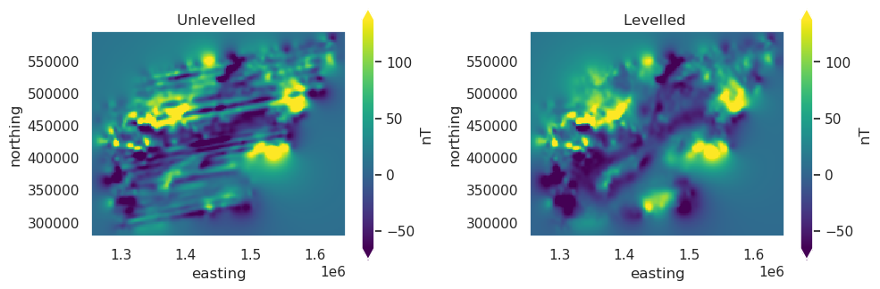
fig, axs = plt.subplots(1, 2, figsize=(10, 6))

vmin, vmax = vd.minmax(
    grid_unlevelled, grid_levelled, min_percentile=2, max_percentile=98
)

grid_unlevelled.plot(
    ax=axs[0],
    cbar_kwargs={
        "shrink": 0.5,
        "label": "nT",
    },
    vmin=vmin,
    vmax=vmax,
)
axs[0].set_title("Unlevelled ")
axs[0].set_aspect("equal")

grid_levelled.plot(
    ax=axs[1],
    cbar_kwargs={
        "shrink": 0.5,
        "label": "nT",
    },
    vmin=vmin,
    vmax=vmax,
)
axs[1].set_title("Levelled ")
axs[1].set_aspect("equal")

plt.tight_layout()
plt.show()
Compute power spectra#
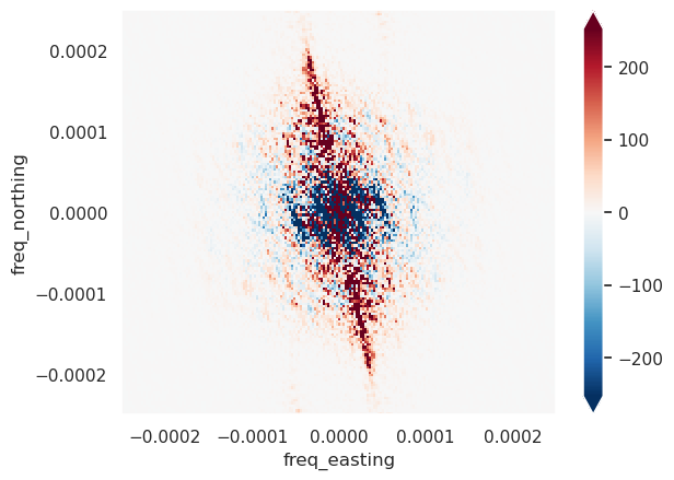
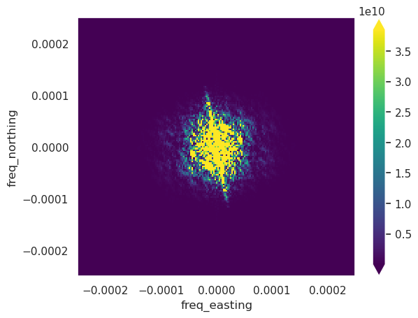
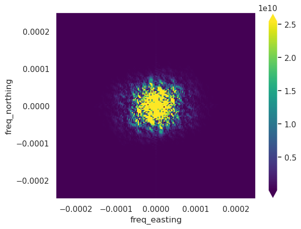
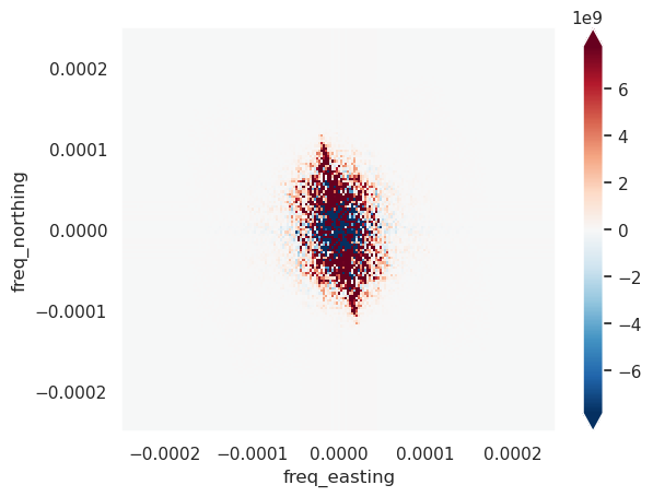
Power spectra of the unlevelled and levelled grids should show if there is a dominant angle of high power, which likely corresponds to levelling errors between lines.
[15]:
powerspec_unlevelled = xrft.power_spectrum(grid_unlevelled)
powerspec_unlevelled.plot(
    robust=True,
)
[15]:
<matplotlib.collections.QuadMesh at 0x7fb46fada5d0>
[16]:
powerspec_levelled = xrft.power_spectrum(grid_levelled)
powerspec_levelled.plot(
    robust=True,
)
[16]:
<matplotlib.collections.QuadMesh at 0x7fb46f997ed0>
Below we show the power spectra differences of the above two plots.
[17]:
(powerspec_unlevelled - powerspec_levelled).plot(
    robust=True,
)
[17]:
<matplotlib.collections.QuadMesh at 0x7fb46f899090>
Use spatial derivatives to assess levelling performance#
[18]:
hg_unlevelled = airbornegeo.filter_grid(
    grid_unlevelled, filter_type="horizontal_gradient"
)
hg_levelled = airbornegeo.filter_grid(grid_levelled, filter_type="horizontal_gradient")
[19]:
fig, axs = plt.subplots(1, 2, figsize=(10, 6))

vmin, vmax = vd.minmax(hg_unlevelled, hg_levelled, min_percentile=2, max_percentile=98)

hg_unlevelled.plot(
    ax=axs[0],
    cbar_kwargs={
        "shrink": 0.5,
        "label": "nT/m",
    },
    vmin=vmin,
    vmax=vmax,
)
axs[0].set_title("Unlevelled Horizontal Gradient")
axs[0].set_aspect("equal")

hg_levelled.plot(
    ax=axs[1],
    cbar_kwargs={
        "shrink": 0.5,
        "label": "nT/m",
    },
    vmin=vmin,
    vmax=vmax,
)
axs[1].set_title("Levelled Horizontal Gradient")
axs[1].set_aspect("equal")

plt.tight_layout()
plt.show()
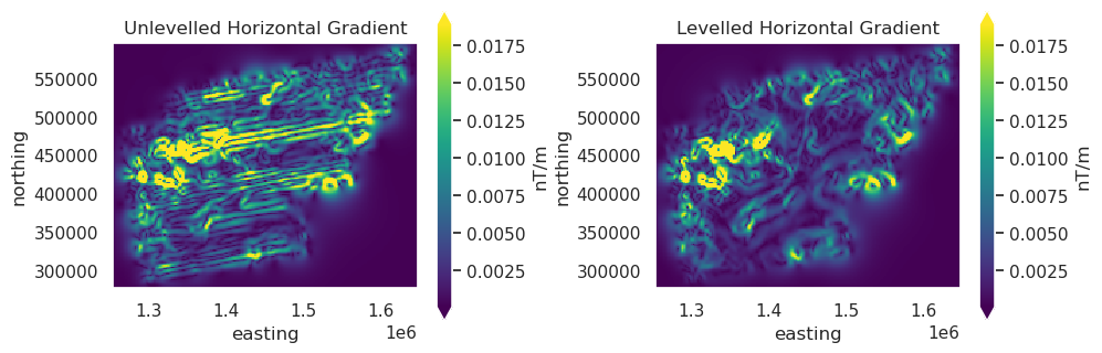
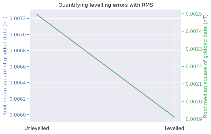
The above plots show the horizontal gradients for the unlevelled and levelled grids. These highlight the levelling errors in the data. These errors appear to be significantly reduced with the levelling. One way to quantify these errors is to compute the RMS of the grid values and the grid with levelling errors will results in more regions of high horizontal gradients, and therefore a higher RMS.
[20]:
airbornegeo.rmse(hg_unlevelled), airbornegeo.rmse(hg_unlevelled, as_median=True)
[20]:
(np.float64(0.007249995388034346), np.float64(0.0024966570729831696))
[21]:
airbornegeo.rmse(hg_levelled), airbornegeo.rmse(hg_levelled, as_median=True)
[21]:
(np.float64(0.005969627985484854), np.float64(0.0019099994766598))
[22]:
fig, ax = plt.subplots(1, 1, sharex=True)
ax.plot(
    ["Unlevelled", "Levelled"],
    [airbornegeo.rmse(hg_unlevelled), airbornegeo.rmse(hg_levelled)],
    c="b",
)
ax.set_ylabel("Root mean square of gridded data (nT)", color="b")
ax.tick_params(axis="y", colors="b", which="both")

ax2 = ax.twinx()
ax2.plot(
    ["Unlevelled", "Levelled"],
    [
        airbornegeo.rmse(hg_unlevelled, as_median=True),
        airbornegeo.rmse(hg_levelled, as_median=True),
    ],
    c="g",
)
ax2.grid(visible=False)
ax2.set_ylabel("Root median square of gridded data (nT)", color="g")
ax2.tick_params(axis="y", colors="g", which="both")

plt.title("Quantifying levelling errors with RMS");
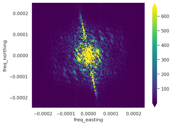
Additionally, we can plot the power spectra of the horizontal gradients of the levelled and unlevelled data. These show a single angle of high power in the data, which is from the levelling errors.
[23]:
powerspec_unlevelled = xrft.power_spectrum(hg_unlevelled)
powerspec_unlevelled.plot(
    robust=True,
)
[23]:
<matplotlib.collections.QuadMesh at 0x7fb46f5d6210>
[24]:
powerspec_levelled = xrft.power_spectrum(hg_levelled)
powerspec_levelled.plot(
    robust=True,
)
[24]:
<matplotlib.collections.QuadMesh at 0x7fb46f47b750>
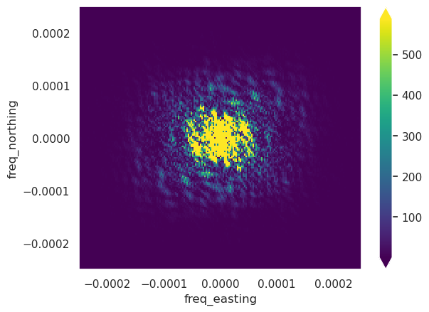
Below we show the power spectra differences of the above two plots.
[25]:
(powerspec_unlevelled - powerspec_levelled).plot(
    robust=True,
)
[25]:
<matplotlib.collections.QuadMesh at 0x7fb46f374910>