1. Vertical acceleration correction#
[1]:
import cmocean
import matplotlib.pyplot as plt
import pandas as pd
import seaborn as sns
import verde as vd

import airbornegeo
/home/sungw937/airbornegeo/.pixi/envs/default/lib/python3.14/site-packages/tqdm/auto.py:21: TqdmWarning: IProgress not found. Please update jupyter and ipywidgets. See https://ipywidgets.readthedocs.io/en/stable/user_install.html
  from .autonotebook import tqdm as notebook_tqdm
1.1. Load data#
This is a subset of the BAS AGAP survey over Antarctica’s Gamburtsev Subglacial Mountains. The file is downloaded and subset in the notebook AGAP_gravity_survey. It has a pre-computed vertical acceleration correction, which we will compare our computed values to.
[2]:
data_df = pd.read_csv("data/AGAP_gravity_survey.csv")
print(data_df.columns)
data_df.head()
Index(['Lon', 'Lat', 'Height_WGS1984', 'Date', 'Time', 'ST', 'CC', 'RB',
       'XACC', 'LACC', 'Still', 'Base', 'ST_real', 'Beam_vel', 'rec_grav',
       'Abs_grav', 'VaccCor', 'EotvosCor', 'LatCor', 'FaCor', 'HaccCor',
       'Free_air', 'FAA_filt', 'FAA_clip', 'Level_cor', 'FAA_level',
       'Fa_4600m', 'easting', 'northing', 'line_name', 'line', 'unixtime'],
      dtype='str')
[2]:
| Lon | Lat | Height_WGS1984 | Date | Time | ST | CC | RB | XACC | LACC | ... | FAA_filt | FAA_clip | Level_cor | FAA_level | Fa_4600m | easting | northing | line_name | line | unixtime | |
|---|---|---|---|---|---|---|---|---|---|---|---|---|---|---|---|---|---|---|---|---|---|
| 0 | 77.252450 | -80.583923 | 4156.1 | 2008-12-17 | 0 days 09:42:48 | 11934.47 | 2.61 | -659.0 | -49.0 | 273.0 | ... | 49.38 | 49.38 | 7.03 | 42.4 | 40.8 | 1.000024e+06 | 226237.330771 | 11_DA500 | 1 | 1.229507e+09 |
| 1 | 77.252672 | -80.583377 | 4156.0 | 2008-12-17 | 0 days 09:42:49 | 11934.47 | 2.72 | -368.6 | -321.0 | 230.0 | ... | 49.45 | 49.45 | 7.04 | 42.4 | 40.8 | 1.000083e+06 | 226246.631269 | 11_DA500 | 1 | 1.229507e+09 |
| 2 | 77.252901 | -80.582831 | 4156.1 | 2008-12-17 | 0 days 09:42:50 | 11888.95 | -2.08 | 703.1 | 433.0 | 146.0 | ... | 49.52 | 49.52 | 7.04 | 42.5 | 40.9 | 1.000142e+06 | 226255.809132 | 11_DA500 | 1 | 1.229507e+09 |
| 3 | 77.253131 | -80.582285 | 4156.4 | 2008-12-17 | 0 days 09:42:51 | 11888.95 | 0.50 | 625.1 | 566.0 | 223.0 | ... | 49.58 | 49.58 | 7.03 | 42.5 | 40.9 | 1.000201e+06 | 226264.969079 | 11_DA500 | 1 | 1.229507e+09 |
| 4 | 77.253358 | -80.581740 | 4156.6 | 2008-12-17 | 0 days 09:42:52 | 11888.95 | -1.73 | 575.1 | 108.0 | 205.0 | ... | 49.65 | 49.65 | 7.04 | 42.6 | 41.0 | 1.000260e+06 | 226274.156809 | 11_DA500 | 1 | 1.229507e+09 |
5 rows × 32 columns
[11]:
data_df["distance_along_line"] = airbornegeo.along_track_distance(
    data_df,
    groupby_column="line",
)
[12]:
# get only the raw columns
# we will perform the corrections ourselves and compare to their values
data_df = data_df[
    [
        "VaccCor",
        "Lon",
        "Lat",
        "Height_WGS1984",
        "easting",
        "northing",
        "unixtime",
        "line",
        "distance_along_line",
    ]
]
data_df.head()
[12]:
| VaccCor | Lon | Lat | Height_WGS1984 | easting | northing | unixtime | line | distance_along_line | |
|---|---|---|---|---|---|---|---|---|---|
| 0 | 5826.01 | 77.252450 | -80.583923 | 4156.1 | 1.000024e+06 | 226237.330771 | 1.229507e+09 | 1 | 0.000000 |
| 1 | 19948.92 | 77.252672 | -80.583377 | 4156.0 | 1.000083e+06 | 226246.631269 | 1.229507e+09 | 1 | 59.842447 |
| 2 | 16840.24 | 77.252901 | -80.582831 | 4156.1 | 1.000142e+06 | 226255.809132 | 1.229507e+09 | 1 | 119.693401 |
| 3 | -2695.10 | 77.253131 | -80.582285 | 4156.4 | 1.000201e+06 | 226264.969079 | 1.229507e+09 | 1 | 179.545645 |
| 4 | 4457.47 | 77.253358 | -80.581740 | 4156.6 | 1.000260e+06 | 226274.156809 | 1.229507e+09 | 1 | 239.285174 |
1.2. Vertical acceleration#
[16]:
data_df["vertical_acceleration"] = airbornegeo.vertical_acceleration(
    data_df,
    groupby_column="line",
    time_column="unixtime",
    height_column="Height_WGS1984",
    smoothing_window=3,
    time_threshold=10,
)

# convert from m/s^2 to mGals
data_df["vertical_acceleration"] *= 10**5
data_df.head()
Segments: 100%|██████████| 167/167 [00:00<00:00, 2031.82it/s]
[16]:
| VaccCor | Lon | Lat | Height_WGS1984 | easting | northing | unixtime | line | distance_along_line | vertical_acceleration | |
|---|---|---|---|---|---|---|---|---|---|---|
| 0 | 5826.01 | 77.252450 | -80.583923 | 4156.1 | 1.000024e+06 | 226237.330771 | 1.229507e+09 | 1 | 0.000000 | 10000.0 |
| 1 | 19948.92 | 77.252672 | -80.583377 | 4156.0 | 1.000083e+06 | 226246.631269 | 1.229507e+09 | 1 | 59.842447 | 12500.0 |
| 2 | 16840.24 | 77.252901 | -80.582831 | 4156.1 | 1.000142e+06 | 226255.809132 | 1.229507e+09 | 1 | 119.693401 | 12500.0 |
| 3 | -2695.10 | 77.253131 | -80.582285 | 4156.4 | 1.000201e+06 | 226264.969079 | 1.229507e+09 | 1 | 179.545645 | 10000.0 |
| 4 | 4457.47 | 77.253358 | -80.581740 | 4156.6 | 1.000260e+06 | 226274.156809 | 1.229507e+09 | 1 | 239.285174 | 7500.0 |
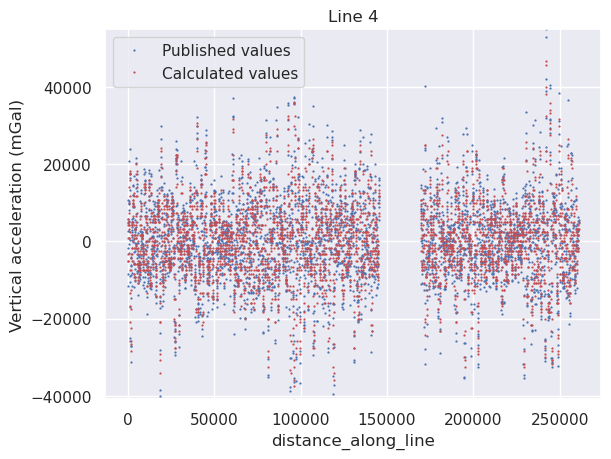
1.3. Compare the results#
[17]:
df = data_df[data_df.line == 4]
ylim = vd.minmax(df.VaccCor)
ax = df.plot.line(
    "distance_along_line",
    "VaccCor",
    style="bp",
    ms=0.6,
    label="Published values",
    title=f"Line {df.line.unique()[0]}",
    ylim=ylim,
)
ax = df.plot.line(
    "distance_along_line",
    "vertical_acceleration",
    style="rp",
    ms=0.6,
    title=f"Line {df.line.unique()[0]}",
    label="Calculated values",
    ax=ax,
    ylim=ylim,
)
ax.set_ylabel("Vertical acceleration (mGal)")
[17]:
Text(0, 0.5, 'Vertical acceleration (mGal)')
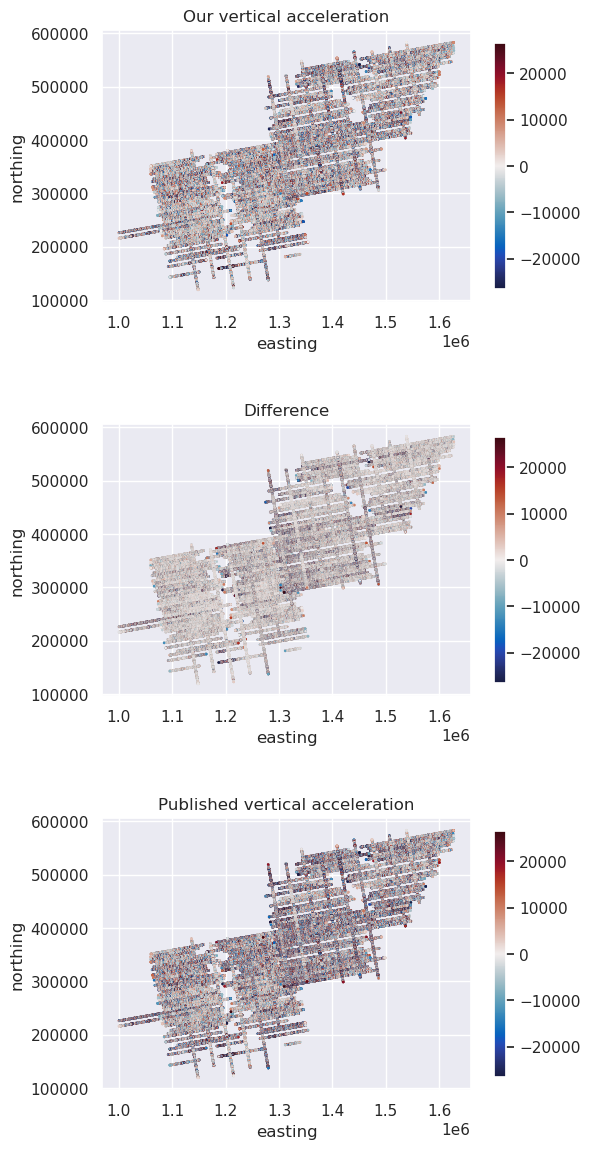
[18]:
data_df["difference"] = data_df["VaccCor"] - data_df["vertical_acceleration"]
[19]:
fig, axs = plt.subplots(3, 1, figsize=(6, 12))

max_abs = vd.maxabs(data_df.VaccCor, percentile=95)

ax = data_df.plot.scatter(
    "easting",
    "northing",
    c="vertical_acceleration",
    s=0.6,
    ax=axs[0],
    cmap=cmocean.cm.balance,
    vmin=-max_abs,
    vmax=max_abs,
    colorbar=False,
    title="Our vertical acceleration",
)
ax.set_aspect("equal")
plt.colorbar(ax.collections[0], ax=ax, shrink=0.8)

ax = data_df.plot.scatter(
    "easting",
    "northing",
    c="difference",
    s=0.6,
    ax=axs[1],
    cmap=cmocean.cm.balance,
    vmin=-max_abs,
    vmax=max_abs,
    colorbar=False,
    title="Difference",
)
ax.set_aspect("equal")
plt.colorbar(ax.collections[0], ax=ax, shrink=0.8)

ax = data_df.plot.scatter(
    "easting",
    "northing",
    c="VaccCor",
    s=0.6,
    ax=axs[2],
    cmap=cmocean.cm.balance,
    vmin=-max_abs,
    vmax=max_abs,
    colorbar=False,
    title="Published vertical acceleration",
)
ax.set_aspect("equal")
plt.colorbar(ax.collections[0], ax=ax, shrink=0.8)

plt.tight_layout()
plt.show()
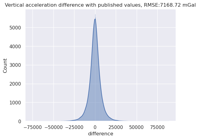
[20]:
sns.histplot((data_df.difference), kde=True)
plt.title(
    f"Vertical acceleration difference with published values, RMSE:{round(airbornegeo.rmse(data_df.difference), 2)} mGal"
)
plt.show()