2. Eotvos correction#
The Eotvos correction is a necessary correction to apply for any gravity surveys conducted on a moving platform, such as a ship or airplane. The correction accounts for the relative motion between the vehicle and the Earth’s surface, which generates an additional centrifugal force known as the Eotvos effect. We offer several methods of computing the correction, which we show here, generally from simpliest to most complex.
[1]:
# %load_ext autoreload
# %autoreload 2

import pandas as pd
import plotly.io as pio
import verde as vd

import airbornegeo

pio.renderers.default = "notebook"
/home/sungw937/airbornegeo/.pixi/envs/default/lib/python3.14/site-packages/tqdm/auto.py:21: TqdmWarning: IProgress not found. Please update jupyter and ipywidgets. See https://ipywidgets.readthedocs.io/en/stable/user_install.html
  from .autonotebook import tqdm as notebook_tqdm
2.1. Load data#
This is a subset of the BAS AGAP survey over Antarctica’s Gamburtsev Subglacial Mountains. The file is downloaded and subset in the notebook AGAP_gravity_survey. It has a pre-computed Eotvos correction, which we will compare our computed values to.
[2]:
data_df = pd.read_csv("data/AGAP_gravity_survey.csv")
print(data_df.columns)
data_df.head()
Index(['Lon', 'Lat', 'Height_WGS1984', 'Date', 'Time', 'ST', 'CC', 'RB',
       'XACC', 'LACC', 'Still', 'Base', 'ST_real', 'Beam_vel', 'rec_grav',
       'Abs_grav', 'VaccCor', 'EotvosCor', 'LatCor', 'FaCor', 'HaccCor',
       'Free_air', 'FAA_filt', 'FAA_clip', 'Level_cor', 'FAA_level',
       'Fa_4600m', 'easting', 'northing', 'line_name', 'line', 'unixtime'],
      dtype='str')
[2]:
| Lon | Lat | Height_WGS1984 | Date | Time | ST | CC | RB | XACC | LACC | ... | FAA_filt | FAA_clip | Level_cor | FAA_level | Fa_4600m | easting | northing | line_name | line | unixtime | |
|---|---|---|---|---|---|---|---|---|---|---|---|---|---|---|---|---|---|---|---|---|---|
| 0 | 77.252450 | -80.583923 | 4156.1 | 2008-12-17 | 0 days 09:42:48 | 11934.47 | 2.61 | -659.0 | -49.0 | 273.0 | ... | 49.38 | 49.38 | 7.03 | 42.4 | 40.8 | 1.000024e+06 | 226237.330771 | 11_DA500 | 1 | 1.229507e+09 |
| 1 | 77.252672 | -80.583377 | 4156.0 | 2008-12-17 | 0 days 09:42:49 | 11934.47 | 2.72 | -368.6 | -321.0 | 230.0 | ... | 49.45 | 49.45 | 7.04 | 42.4 | 40.8 | 1.000083e+06 | 226246.631269 | 11_DA500 | 1 | 1.229507e+09 |
| 2 | 77.252901 | -80.582831 | 4156.1 | 2008-12-17 | 0 days 09:42:50 | 11888.95 | -2.08 | 703.1 | 433.0 | 146.0 | ... | 49.52 | 49.52 | 7.04 | 42.5 | 40.9 | 1.000142e+06 | 226255.809132 | 11_DA500 | 1 | 1.229507e+09 |
| 3 | 77.253131 | -80.582285 | 4156.4 | 2008-12-17 | 0 days 09:42:51 | 11888.95 | 0.50 | 625.1 | 566.0 | 223.0 | ... | 49.58 | 49.58 | 7.03 | 42.5 | 40.9 | 1.000201e+06 | 226264.969079 | 11_DA500 | 1 | 1.229507e+09 |
| 4 | 77.253358 | -80.581740 | 4156.6 | 2008-12-17 | 0 days 09:42:52 | 11888.95 | -1.73 | 575.1 | 108.0 | 205.0 | ... | 49.65 | 49.65 | 7.04 | 42.6 | 41.0 | 1.000260e+06 | 226274.156809 | 11_DA500 | 1 | 1.229507e+09 |
5 rows × 32 columns
[3]:
data_df["distance_along_line"] = airbornegeo.along_track_distance(
    data_df,
    groupby_column="line",
)
[4]:
# get only the raw columns
# we will perform the corrections ourselves and compare to their values
data_df = data_df[
    [
        "EotvosCor",
        "Lon",
        "Lat",
        "Height_WGS1984",
        "easting",
        "northing",
        "unixtime",
        "line",
        "distance_along_line",
    ]
]
data_df.head()
[4]:
| EotvosCor | Lon | Lat | Height_WGS1984 | easting | northing | unixtime | line | distance_along_line | |
|---|---|---|---|---|---|---|---|---|---|
| 0 | 68.15 | 77.252450 | -80.583923 | 4156.1 | 1.000024e+06 | 226237.330771 | 1.229507e+09 | 1 | 0.000000 |
| 1 | 68.37 | 77.252672 | -80.583377 | 4156.0 | 1.000083e+06 | 226246.631269 | 1.229507e+09 | 1 | 59.842447 |
| 2 | 68.37 | 77.252901 | -80.582831 | 4156.1 | 1.000142e+06 | 226255.809132 | 1.229507e+09 | 1 | 119.693401 |
| 3 | 68.16 | 77.253131 | -80.582285 | 4156.4 | 1.000201e+06 | 226264.969079 | 1.229507e+09 | 1 | 179.545645 |
| 4 | 68.12 | 77.253358 | -80.581740 | 4156.6 | 1.000260e+06 | 226274.156809 | 1.229507e+09 | 1 | 239.285174 |
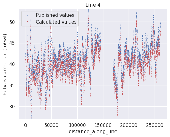
2.2. Eotvos correction following Glicken 1962#
The most simple method of calculating the Eotvos correction is the Glicken 1962 formula, which depends on only the latitudes, the track angle, and the ground speed. This approximation ignores the effects of aircraft altitude, and the flattening of the ellipsoid. It does this by assuming heights are neglible compared to the radius of the Earth, and the change in Earth radius with latitude (flatenning) is also negligible, so the mean radius of the Earth is used. This results in a simple formula of
E = 7.503 V \cos\phi \sin\tau + 0.00415V^2
where \(V\) is the ground speed of the aircraft, \(\phi\) is the geodetic latitude, and \(\tau\) is the track angle.
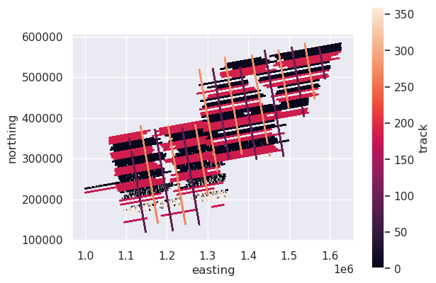
The track angle is similar to the aircraft’s heading. The heading is the angle the nose of the plane points, which due to wind, can differ from the angle the path of the plane makes. This is in degrees clockwise from geographic (true) north.
By setting ellipsoid=True in the below function, we calculate the track using the WGS84 ellipsoid, instead of using a simplified spheric model of the Earth. It is more accurate, but a bit slower to compute.
[5]:
data_df["track"] = airbornegeo.track(
    data_df,
    latitude_column="Lat",
    longitude_column="Lon",
    groupby_column="line",
    ellipsoid=False,  # setting this to False is faster but less accurate
)
data_df.head()
Segments: 100%|██████████| 100/100 [00:00<00:00, 1707.48it/s]
[5]:
| EotvosCor | Lon | Lat | Height_WGS1984 | easting | northing | unixtime | line | distance_along_line | track | |
|---|---|---|---|---|---|---|---|---|---|---|
| 0 | 68.15 | 77.252450 | -80.583923 | 4156.1 | 1.000024e+06 | 226237.330771 | 1.229507e+09 | 1 | 0.000000 | 3.925778 |
| 1 | 68.37 | 77.252672 | -80.583377 | 4156.0 | 1.000083e+06 | 226246.631269 | 1.229507e+09 | 1 | 59.842447 | 3.805916 |
| 2 | 68.37 | 77.252901 | -80.582831 | 4156.1 | 1.000142e+06 | 226255.809132 | 1.229507e+09 | 1 | 119.693401 | 3.925778 |
| 3 | 68.16 | 77.253131 | -80.582285 | 4156.4 | 1.000201e+06 | 226264.969079 | 1.229507e+09 | 1 | 179.545645 | 3.943093 |
| 4 | 68.12 | 77.253358 | -80.581740 | 4156.6 | 1.000260e+06 | 226274.156809 | 1.229507e+09 | 1 | 239.285174 | 3.899163 |
[6]:
ax = data_df.plot.scatter(
    "easting",
    "northing",
    c="track",
    s=0.2,
)
ax.set_aspect("equal")
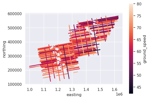
The Glicken formulation also requiresthe ground speed of the aircraft. The below function ground_speed calculates the relative distance between successive rows in the dataframe. This assumes the dataframe is sorted by line, and then by time. From the relative distance, it then calculate the ground speed of the aircraft.
[7]:
data_df["ground_speed"] = airbornegeo.ground_speed(
    data_df,
    easting_column="easting",
    northing_column="northing",
    time_column="unixtime",
    groupby_column="line",
)
data_df.head()
Segments: 100%|██████████| 100/100 [00:00<00:00, 6647.60it/s]
Segments: 100%|██████████| 100/100 [00:00<00:00, 2661.61it/s]
[7]:
| EotvosCor | Lon | Lat | Height_WGS1984 | easting | northing | unixtime | line | distance_along_line | track | ground_speed | |
|---|---|---|---|---|---|---|---|---|---|---|---|
| 0 | 68.15 | 77.252450 | -80.583923 | 4156.1 | 1.000024e+06 | 226237.330771 | 1.229507e+09 | 1 | 0.000000 | 3.925778 | 59.842447 |
| 1 | 68.37 | 77.252672 | -80.583377 | 4156.0 | 1.000083e+06 | 226246.631269 | 1.229507e+09 | 1 | 59.842447 | 3.805916 | 59.846701 |
| 2 | 68.37 | 77.252901 | -80.582831 | 4156.1 | 1.000142e+06 | 226255.809132 | 1.229507e+09 | 1 | 119.693401 | 3.925778 | 59.851599 |
| 3 | 68.16 | 77.253131 | -80.582285 | 4156.4 | 1.000201e+06 | 226264.969079 | 1.229507e+09 | 1 | 179.545645 | 3.943093 | 59.795886 |
| 4 | 68.12 | 77.253358 | -80.581740 | 4156.6 | 1.000260e+06 | 226274.156809 | 1.229507e+09 | 1 | 239.285174 | 3.899163 | 59.740782 |
[8]:
ax = data_df.plot.scatter(
    "easting",
    "northing",
    c="ground_speed",
    s=0.2,
)
ax.set_aspect("equal")
[9]:
data_df["eotvos_correction_glicken"] = airbornegeo.eotvos_correction_glicken(
    data_df.Lat.values,
    data_df.track.values,
    data_df.ground_speed.values,
)
data_df.head()
[9]:
| EotvosCor | Lon | Lat | Height_WGS1984 | easting | northing | unixtime | line | distance_along_line | track | ground_speed | eotvos_correction_glicken | |
|---|---|---|---|---|---|---|---|---|---|---|---|---|
| 0 | 68.15 | 77.252450 | -80.583923 | 4156.1 | 1.000024e+06 | 226237.330771 | 1.229507e+09 | 1 | 0.000000 | 3.925778 | 59.842447 | 65.984990 |
| 1 | 68.37 | 77.252672 | -80.583377 | 4156.0 | 1.000083e+06 | 226246.631269 | 1.229507e+09 | 1 | 59.842447 | 3.805916 | 59.846701 | 65.696167 |
| 2 | 68.37 | 77.252901 | -80.582831 | 4156.1 | 1.000142e+06 | 226255.809132 | 1.229507e+09 | 1 | 119.693401 | 3.925778 | 59.851599 | 66.004804 |
| 3 | 68.16 | 77.253131 | -80.582285 | 4156.4 | 1.000201e+06 | 226264.969079 | 1.229507e+09 | 1 | 179.545645 | 3.943093 | 59.795886 | 65.934659 |
| 4 | 68.12 | 77.253358 | -80.581740 | 4156.6 | 1.000260e+06 | 226274.156809 | 1.229507e+09 | 1 | 239.285174 | 3.899163 | 59.740782 | 65.713724 |
[10]:
ax = data_df.plot.scatter(
    "easting",
    "northing",
    c="eotvos_correction_glicken",
    s=0.2,
)
ax.set_aspect("equal")

[11]:
df = data_df[data_df.line == 4]
ylim = vd.minmax(df.EotvosCor)
ax = df.plot.line(
    "distance_along_line",
    "EotvosCor",
    style="bp",
    ms=0.6,
    label="Published values",
    title=f"Line {df.line.unique()[0]}",
    ylim=ylim,
)
ax = df.plot.line(
    "distance_along_line",
    "eotvos_correction_glicken",
    style="rp",
    ms=0.6,
    title=f"Line {df.line.unique()[0]}",
    label="Calculated values",
    ax=ax,
    ylim=ylim,
)
ax.set_ylabel("Eotvos correction (mGal)")
[11]:
Text(0, 0.5, 'Eotvos correction (mGal)')
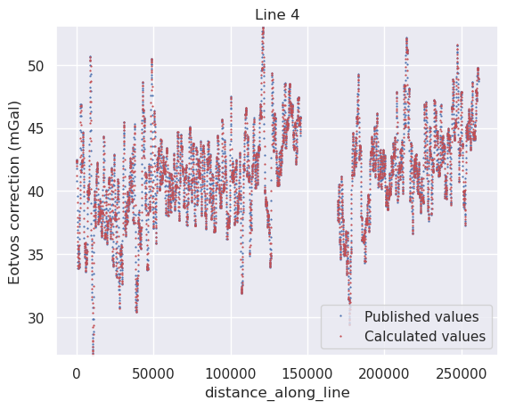
2.3. Eotvos correction following Harlan 1968#
Another common method to compute the correction is from Harlan 1968. The paper offers several equations, but first we will follow equation 15.
2.3.1. Equation 15:#
This formulation requires the aircraft latitude, longtide, time (to calculate time derivatives) and height.
E = \frac{V_N^2}{a} [ 1 + \frac{h}{a} + f (2-3\sin^{2}\phi) ] + \frac{V_E^2}{a} [ 1 + \frac{h}{a} - f \sin^{2}\phi) ] + 2 V_E \omega \cos \phi (1 + \frac{h}{a})
where \(V_N\), \(V_E\), \(h\), and \(\phi\), $ are the aircraft’s eastward and northward velocities, height, and geodetic latitude, and \(a\), \(f\), and \(\omega\) are the ellipsoid’s semimajor axis, flattening, and rotation rate.
V_N = r' \dot{\phi_{c}} sec(D)
V_E = r' \dot{l} cos(\phi_{c})
where \(r'\) is the ellipsoid’s geocentric radius at the latitude of the aircraft, \(l\) is the aircraft’s longitude, \(\phi_{c}\) is the geocentric radius of the aircraft, \(\dot{\phi_{c}}\) is the first time derivative of the geocentric radius of the aircraft, and \(D\) is the deviation between the aircraft’s geodetic latitude and geocentric latitude.
Compared to the Glicken formulation, it is more exact since it accounts for aircraft height as well as the flattening of the ellipsoid. However it still makes a few assumptions which simplify the calculations. These include a simplification for the deviation between geocentric and geodetic latitudes, and thus the time derivatives of this deviation, as well as a simplification of the geocentric radius, and thus the time derivatives of the geocentric radius.
[33]:
data_df["eotvos_correction_harlan"] = airbornegeo.eotvos_correction_harlan(
    data_df.Lat.values,
    data_df.Lon.values,
    data_df.unixtime.values,
    data_df.Height_WGS1984.values,
)
data_df.head()
[33]:
| EotvosCor | Lon | Lat | Height_WGS1984 | easting | northing | unixtime | line | distance_along_line | track | ground_speed | eotvos_correction_glicken | eotvos_correction_harlan | velocity_longitudinal | velocity_latitudinal | eotvos_correction_harlan_velocity | eotvos_correction_harlan_at_altitude | dif | |
|---|---|---|---|---|---|---|---|---|---|---|---|---|---|---|---|---|---|---|
| 0 | 68.15 | 77.252450 | -80.583923 | 4156.1 | 1.000024e+06 | 226237.330771 | 1.229507e+09 | 1 | 0.000000 | 3.925778 | 59.842447 | 65.984990 | 68.079899 | 0.000222 | 0.000546 | 68.079384 | 68.079384 | 0.000515 |
| 1 | 68.37 | 77.252672 | -80.583377 | 4156.0 | 1.000083e+06 | 226246.631269 | 1.229507e+09 | 1 | 59.842447 | 3.805916 | 59.846701 | 65.696167 | 68.241925 | 0.000225 | 0.000546 | 68.241409 | 68.241409 | 0.000516 |
| 2 | 68.37 | 77.252901 | -80.582831 | 4156.1 | 1.000142e+06 | 226255.809132 | 1.229507e+09 | 1 | 119.693401 | 3.925778 | 59.851599 | 66.004804 | 68.427131 | 0.000229 | 0.000546 | 68.426614 | 68.426614 | 0.000516 |
| 3 | 68.16 | 77.253131 | -80.582285 | 4156.4 | 1.000201e+06 | 226264.969079 | 1.229507e+09 | 1 | 179.545645 | 3.943093 | 59.795886 | 65.934659 | 68.275851 | 0.000229 | 0.000546 | 68.275336 | 68.275336 | 0.000515 |
| 4 | 68.12 | 77.253358 | -80.581740 | 4156.6 | 1.000260e+06 | 226274.156809 | 1.229507e+09 | 1 | 239.285174 | 3.899163 | 59.740782 | 65.713724 | 68.147679 | 0.000228 | 0.000545 | 68.147164 | 68.147164 | 0.000514 |
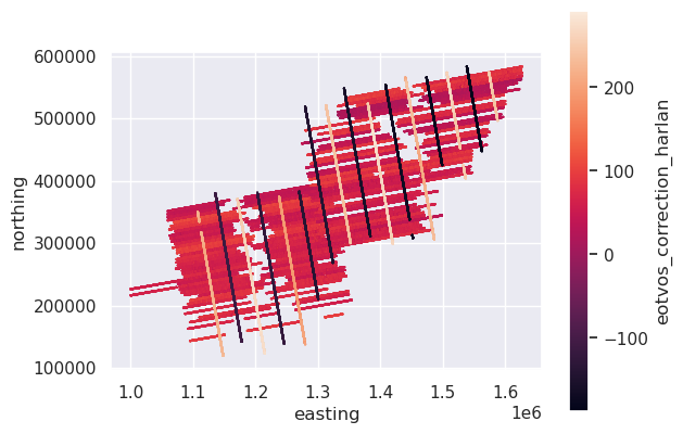
[34]:
ax = data_df.plot.scatter(
    "easting",
    "northing",
    c="eotvos_correction_harlan",
    s=0.2,
)
ax.set_aspect("equal")
[35]:
df = data_df[data_df.line == 4]
ylim = vd.minmax(df.EotvosCor)
ax = df.plot.line(
    "distance_along_line",
    "EotvosCor",
    style="bp",
    ms=0.6,
    label="Published values",
    title=f"Line {df.line.unique()[0]}",
    ylim=ylim,
)
ax = df.plot.line(
    "distance_along_line",
    "eotvos_correction_harlan",
    style="rp",
    ms=0.6,
    title=f"Line {df.line.unique()[0]}",
    label="Calculated values",
    ax=ax,
    ylim=ylim,
)
ax.set_ylabel("Eotvos correction (mGal)")
[35]:
Text(0, 0.5, 'Eotvos correction (mGal)')