1. Levelling to a grid#
[1]:
# %load_ext autoreload
# %autoreload 2

import boule
import cmocean
import numpy as np
import pandas as pd
import polartoolkit as ptk
import verde as vd

import airbornegeo
/home/sungw937/airbornegeo/.pixi/envs/default/lib/python3.14/site-packages/tqdm/auto.py:21: TqdmWarning: IProgress not found. Please update jupyter and ipywidgets. See https://ipywidgets.readthedocs.io/en/stable/user_install.html
  from .autonotebook import tqdm as notebook_tqdm
1.1. Load survey data#
This is a subset of the BAS AGAP survey over Antarctica’s Gamburtsev Subglacial Mountains. The file is download and subset in the notebook AGAP_gravity_survey, and the BAS processing steps are repeated in the notebook processing_AGAP_gravity_survey.
[10]:
data_df = pd.read_csv("data/AGAP_gravity_survey_processed.csv")
data_df = data_df[
    [
        "easting",
        "northing",
        "height",
        "line",
        "unixtime",
        "distance_along_line",
        "grav_disturbance_filt",
    ]
]
data_df.head()
[10]:
| easting | northing | height | line | unixtime | distance_along_line | grav_disturbance_filt | |
|---|---|---|---|---|---|---|---|
| 0 | 1.000024e+06 | 226237.330771 | 4156.1 | 1 | 1.229507e+09 | 0.000000 | 49.38 |
| 1 | 1.000083e+06 | 226246.631269 | 4156.0 | 1 | 1.229507e+09 | 59.842447 | 49.45 |
| 2 | 1.000142e+06 | 226255.809132 | 4156.1 | 1 | 1.229507e+09 | 119.693401 | 49.52 |
| 3 | 1.000201e+06 | 226264.969079 | 4156.4 | 1 | 1.229507e+09 | 179.545645 | 49.58 |
| 4 | 1.000260e+06 | 226274.156809 | 4156.6 | 1 | 1.229507e+09 | 239.285174 | 49.65 |
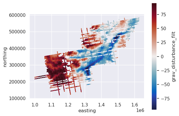
[12]:
# plot the data
max_abs = vd.maxabs(data_df.grav_disturbance_filt, percentile=95)
ax = data_df.plot.scatter(
    "easting",
    "northing",
    c="grav_disturbance_filt",
    s=0.1,
    cmap=cmocean.cm.balance,
    vmin=-max_abs,
    vmax=max_abs,
)
ax.set_aspect("equal")
1.2. Get a grid of gravity disturbance at 10km#
[13]:
# Download satellite gravity data from EIGEN-6C4 model
region = vd.get_region((data_df.easting, data_df.northing))
eigen = ptk.fetch.gravity(
    version="eigen",
    spacing=5e3,
    region=region,
    epsg="3031",
)
eigen_df = vd.grid_to_table(eigen)
eigen_df = eigen_df.rename(columns={"x": "easting", "y": "northing"})

# reproject from EPSG 3031 to lat lon
eigen_df["lon"], eigen_df["lat"] = airbornegeo.reproject(
    eigen_df.easting,
    eigen_df.northing,
    input_crs="EPSG:3031",
    output_crs="EPSG:4326",
)

# calculated normal gravity at all EIGEN observation locations
eigen_df["normal_gravity"] = boule.WGS84.normal_gravity(
    (None, eigen_df.lat, eigen_df.ellipsoidal_height),
)

# calculate gravity disturbance
eigen_df["disturbance"] = eigen_df.gravity - eigen_df.normal_gravity

# convert to a dataset
eigen_ds = eigen_df.set_index(["northing", "easting"]).to_xarray()

eigen_ds
[13]:
<xarray.Dataset> Size: 479kB
Dimensions:             (northing: 94, easting: 127)
Coordinates:
  * northing            (northing) float64 752B 1.2e+05 1.25e+05 ... 5.85e+05
  * easting             (easting) float64 1kB 1e+06 1.005e+06 ... 1.63e+06
Data variables:
    ellipsoidal_height  (northing, easting) float32 48kB 1e+04 1e+04 ... 1e+04
    gravity             (northing, easting) float32 48kB 9.8e+05 ... 9.797e+05
    lon                 (northing, easting) float64 96kB 83.16 83.19 ... 70.26
    lat                 (northing, easting) float64 96kB -80.75 -80.7 ... -74.16
    normal_gravity      (northing, easting) float64 96kB 9.8e+05 ... 9.798e+05
disturbance (northing, easting) float64 96kB 38.05 38.12 ... -20.55[14]:
eigen_ds.disturbance.plot()
[14]:
<matplotlib.collections.QuadMesh at 0x7f37d1b1ce10>
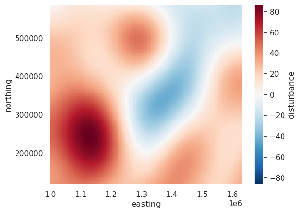
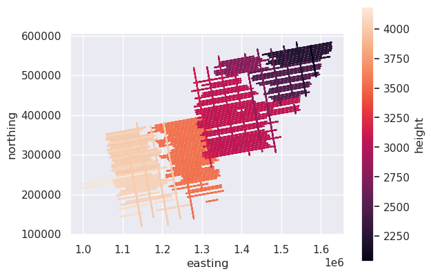
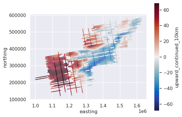
1.3. Upward continue survey data to same height as gravity grid#
In order to accurately compare the survey gravity data to the grid, the gravity data should be upward continued so it’s at the same altitude.
[15]:
# plot the data
ax = data_df.plot.scatter(
    "easting",
    "northing",
    c="height",
    s=0.1,
)
ax.set_aspect("equal")
[16]:
blocked_survey = airbornegeo.block_reduce(
    data_df,
    np.median,
    spacing=1000,
    reduce_by="distance_along_line",
    groupby_column="line",
)
blocked_survey
Segments: 100%|██████████| 100/100 [00:12<00:00, 7.99it/s]
[16]:
| distance_along_line | easting | northing | height | unixtime | grav_disturbance_filt | line | |
|---|---|---|---|---|---|---|---|
| 0 | 477.521406 | 1.000496e+06 | 226310.158049 | 4159.10 | 1.229507e+09 | 49.890 | 1 |
| 1 | 1477.462561 | 1.001484e+06 | 226460.426302 | 4160.30 | 1.229507e+09 | 50.730 | 1 |
| 2 | 2504.019094 | 1.002497e+06 | 226630.494762 | 4156.00 | 1.229507e+09 | 51.090 | 1 |
| 3 | 3518.522095 | 1.003499e+06 | 226786.791629 | 4159.60 | 1.229507e+09 | 51.070 | 1 |
| 4 | 4528.427996 | 1.004498e+06 | 226936.380167 | 4165.70 | 1.229507e+09 | 51.430 | 1 |
| ... | ... | ... | ... | ... | ... | ... | ... |
| 21443 | 74604.147937 | 1.587227e+06 | 500746.382318 | 2091.50 | 1.230382e+09 | -14.050 | 100 |
| 21444 | 75624.848269 | 1.587399e+06 | 499740.258279 | 2105.95 | 1.230382e+09 | -16.245 | 100 |
| 21445 | 76638.943754 | 1.587565e+06 | 498740.092633 | 2110.60 | 1.230382e+09 | -17.580 | 100 |
| 21446 | 77637.520664 | 1.587737e+06 | 497756.392340 | 2113.00 | 1.230382e+09 | -17.820 | 100 |
| 21447 | 78639.391988 | 1.587918e+06 | 496771.090597 | 2115.30 | 1.230382e+09 | -17.180 | 100 |
21448 rows × 7 columns
[17]:
# fit a set of equivalent sources to each line individually
eqs = airbornegeo.eq_sources_1d(
    blocked_survey,
    data_column="grav_disturbance_filt",
    depth="default",
    damping=None,
    block_size=1000,  # for speed, block reduce sources
    groupby_column="line",
)
eqs
Groups: 100%|██████████| 100/100 [00:14<00:00, 7.12it/s]
[17]:
{1: EquivalentSources(block_size=1000),
 2: EquivalentSources(block_size=1000),
 3: EquivalentSources(block_size=1000),
 4: EquivalentSources(block_size=1000),
 5: EquivalentSources(block_size=1000),
 6: EquivalentSources(block_size=1000),
 7: EquivalentSources(block_size=1000),
 8: EquivalentSources(block_size=1000),
 9: EquivalentSources(block_size=1000),
 10: EquivalentSources(block_size=1000),
 11: EquivalentSources(block_size=1000),
 12: EquivalentSources(block_size=1000),
 13: EquivalentSources(block_size=1000),
 14: EquivalentSources(block_size=1000),
 15: EquivalentSources(block_size=1000),
 16: EquivalentSources(block_size=1000),
 17: EquivalentSources(block_size=1000),
 18: EquivalentSources(block_size=1000),
 19: EquivalentSources(block_size=1000),
 20: EquivalentSources(block_size=1000),
 21: EquivalentSources(block_size=1000),
 22: EquivalentSources(block_size=1000),
 23: EquivalentSources(block_size=1000),
 24: EquivalentSources(block_size=1000),
 25: EquivalentSources(block_size=1000),
 26: EquivalentSources(block_size=1000),
 27: EquivalentSources(block_size=1000),
 28: EquivalentSources(block_size=1000),
 29: EquivalentSources(block_size=1000),
 30: EquivalentSources(block_size=1000),
 31: EquivalentSources(block_size=1000),
 32: EquivalentSources(block_size=1000),
 33: EquivalentSources(block_size=1000),
 34: EquivalentSources(block_size=1000),
 35: EquivalentSources(block_size=1000),
 36: EquivalentSources(block_size=1000),
 37: EquivalentSources(block_size=1000),
 38: EquivalentSources(block_size=1000),
 39: EquivalentSources(block_size=1000),
 40: EquivalentSources(block_size=1000),
 41: EquivalentSources(block_size=1000),
 42: EquivalentSources(block_size=1000),
 43: EquivalentSources(block_size=1000),
 44: EquivalentSources(block_size=1000),
 45: EquivalentSources(block_size=1000),
 46: EquivalentSources(block_size=1000),
 47: EquivalentSources(block_size=1000),
 48: EquivalentSources(block_size=1000),
 49: EquivalentSources(block_size=1000),
 50: EquivalentSources(block_size=1000),
 51: EquivalentSources(block_size=1000),
 52: EquivalentSources(block_size=1000),
 53: EquivalentSources(block_size=1000),
 54: EquivalentSources(block_size=1000),
 55: EquivalentSources(block_size=1000),
 56: EquivalentSources(block_size=1000),
 57: EquivalentSources(block_size=1000),
 58: EquivalentSources(block_size=1000),
 59: EquivalentSources(block_size=1000),
 60: EquivalentSources(block_size=1000),
 61: EquivalentSources(block_size=1000),
 62: EquivalentSources(block_size=1000),
 63: EquivalentSources(block_size=1000),
 64: EquivalentSources(block_size=1000),
 65: EquivalentSources(block_size=1000),
 66: EquivalentSources(block_size=1000),
 67: EquivalentSources(block_size=1000),
 68: EquivalentSources(block_size=1000),
 69: EquivalentSources(block_size=1000),
 70: EquivalentSources(block_size=1000),
 71: EquivalentSources(block_size=1000),
 72: EquivalentSources(block_size=1000),
 73: EquivalentSources(block_size=1000),
 74: EquivalentSources(block_size=1000),
 75: EquivalentSources(block_size=1000),
 76: EquivalentSources(block_size=1000),
 77: EquivalentSources(block_size=1000),
 78: EquivalentSources(block_size=1000),
 79: EquivalentSources(block_size=1000),
 80: EquivalentSources(block_size=1000),
 81: EquivalentSources(block_size=1000),
 82: EquivalentSources(block_size=1000),
 83: EquivalentSources(block_size=1000),
 84: EquivalentSources(block_size=1000),
 85: EquivalentSources(block_size=1000),
 86: EquivalentSources(block_size=1000),
 87: EquivalentSources(block_size=1000),
 88: EquivalentSources(block_size=1000),
 89: EquivalentSources(block_size=1000),
 90: EquivalentSources(block_size=1000),
 91: EquivalentSources(block_size=1000),
 92: EquivalentSources(block_size=1000),
 93: EquivalentSources(block_size=1000),
 94: EquivalentSources(block_size=1000),
 95: EquivalentSources(block_size=1000),
 96: EquivalentSources(block_size=1000),
 97: EquivalentSources(block_size=1000),
 98: EquivalentSources(block_size=1000),
 99: EquivalentSources(block_size=1000),
 100: EquivalentSources(block_size=1000)}
[18]:
# upward continue each line to 10 km
blocked_survey["upward_continued_10km"] = airbornegeo.upward_continue_by_line(
    blocked_survey,
    eqs,
    height=10e3,
)
blocked_survey.head()
Groups: 100%|██████████| 100/100 [00:00<00:00, 158.69it/s]
[18]:
| distance_along_line | easting | northing | height | unixtime | grav_disturbance_filt | line | upward_continued_10km | |
|---|---|---|---|---|---|---|---|---|
| 0 | 477.521406 | 1.000496e+06 | 226310.158049 | 4159.1 | 1.229507e+09 | 49.89 | 1 | 40.232278 |
| 1 | 1477.462561 | 1.001484e+06 | 226460.426302 | 4160.3 | 1.229507e+09 | 50.73 | 1 | 40.972657 |
| 2 | 2504.019094 | 1.002497e+06 | 226630.494762 | 4156.0 | 1.229507e+09 | 51.09 | 1 | 41.713109 |
| 3 | 3518.522095 | 1.003499e+06 | 226786.791629 | 4159.6 | 1.229507e+09 | 51.07 | 1 | 42.431563 |
| 4 | 4528.427996 | 1.004498e+06 | 226936.380167 | 4165.7 | 1.229507e+09 | 51.43 | 1 | 43.141623 |
[20]:
# plot the upward continued data
max_abs = vd.maxabs(blocked_survey.upward_continued_10km, percentile=95)
ax = blocked_survey.plot.scatter(
    "easting",
    "northing",
    c="upward_continued_10km",
    s=0.1,
    cmap=cmocean.cm.balance,
    vmin=-max_abs,
    vmax=max_abs,
)
ax.set_aspect("equal")
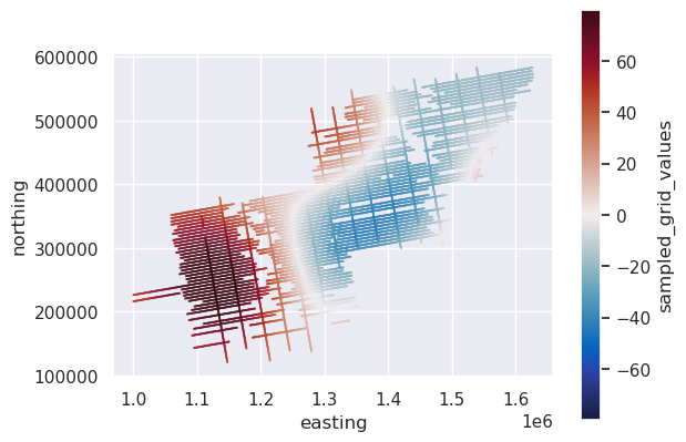
1.3.1. Sample the satellite gravity grid values into the dataframe#
[21]:
# sample grid along lines
blocked_survey["sampled_grid_values"] = airbornegeo.sample_grid(
    blocked_survey,
    eigen_ds.disturbance,
    coord_names=("easting", "northing"),
)
blocked_survey.head()
grdtrack [WARNING]: Some input points were outside the grid domain(s).
[21]:
| distance_along_line | easting | northing | height | unixtime | grav_disturbance_filt | line | upward_continued_10km | sampled_grid_values | |
|---|---|---|---|---|---|---|---|---|---|
| 0 | 477.521406 | 1.000496e+06 | 226310.158049 | 4159.1 | 1.229507e+09 | 49.89 | 1 | 40.232278 | 48.675663 |
| 1 | 1477.462561 | 1.001484e+06 | 226460.426302 | 4160.3 | 1.229507e+09 | 50.73 | 1 | 40.972657 | 48.836891 |
| 2 | 2504.019094 | 1.002497e+06 | 226630.494762 | 4156.0 | 1.229507e+09 | 51.09 | 1 | 41.713109 | 49.005095 |
| 3 | 3518.522095 | 1.003499e+06 | 226786.791629 | 4159.6 | 1.229507e+09 | 51.07 | 1 | 42.431563 | 49.172386 |
| 4 | 4528.427996 | 1.004498e+06 | 226936.380167 | 4165.7 | 1.229507e+09 | 51.43 | 1 | 43.141623 | 49.342525 |
[23]:
# plot the sampled grid values
max_abs = vd.maxabs(blocked_survey.sampled_grid_values, percentile=95)
ax = blocked_survey.plot.scatter(
    "easting",
    "northing",
    c="sampled_grid_values",
    s=0.1,
    cmap=cmocean.cm.balance,
    vmin=-max_abs,
    vmax=max_abs,
)
ax.set_aspect("equal")
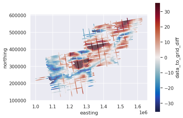
[24]:
# plot the difference
blocked_survey["data_to_grid_diff"] = (
    blocked_survey.upward_continued_10km - blocked_survey.sampled_grid_values
)
max_abs = vd.maxabs(blocked_survey.data_to_grid_diff, percentile=95)
ax = blocked_survey.plot.scatter(
    "easting",
    "northing",
    c="data_to_grid_diff",
    s=0.1,
    cmap=cmocean.cm.balance,
    vmin=-max_abs,
    vmax=max_abs,
)
ax.set_aspect("equal")
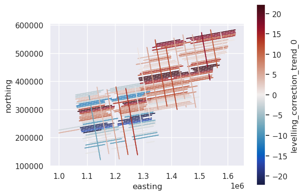
1.4. Level the lines to the grid#
[25]:
blocked_survey["levelled_trend_0"] = airbornegeo.level_to_grid(
    blocked_survey,
    degree=0,  # DC shift
    data_column="upward_continued_10km",
    grid_column="sampled_grid_values",
    groupby_column="line",
)
blocked_survey["levelled_trend_1"] = airbornegeo.level_to_grid(
    blocked_survey,
    degree=1,  # DC shift + tilt
    data_column="upward_continued_10km",
    grid_column="sampled_grid_values",
    groupby_column="line",
)
blocked_survey.head()
[25]:
| distance_along_line | easting | northing | height | unixtime | grav_disturbance_filt | line | upward_continued_10km | sampled_grid_values | data_to_grid_diff | levelled_trend_0 | levelled_trend_1 | |
|---|---|---|---|---|---|---|---|---|---|---|---|---|
| 0 | 477.521406 | 1.000496e+06 | 226310.158049 | 4159.1 | 1.229507e+09 | 49.89 | 1 | 40.232278 | 48.675663 | -8.443385 | 42.596650 | 39.485331 |
| 1 | 1477.462561 | 1.001484e+06 | 226460.426302 | 4160.3 | 1.229507e+09 | 50.73 | 1 | 40.972657 | 48.836891 | -7.864234 | 43.337029 | 40.252951 |
| 2 | 2504.019094 | 1.002497e+06 | 226630.494762 | 4156.0 | 1.229507e+09 | 51.09 | 1 | 41.713109 | 49.005095 | -7.291987 | 44.077481 | 41.021368 |
| 3 | 3518.522095 | 1.003499e+06 | 226786.791629 | 4159.6 | 1.229507e+09 | 51.07 | 1 | 42.431563 | 49.172386 | -6.740823 | 44.795935 | 41.767460 |
| 4 | 4528.427996 | 1.004498e+06 | 226936.380167 | 4165.7 | 1.229507e+09 | 51.43 | 1 | 43.141623 | 49.342525 | -6.200902 | 45.505995 | 42.505032 |
[26]:
# plot the levelling correction
blocked_survey["levelling_correction_trend_0"] = (
    blocked_survey.upward_continued_10km - blocked_survey.levelled_trend_0
)
max_abs = vd.maxabs(blocked_survey.levelling_correction_trend_0, percentile=95)
ax = blocked_survey.plot.scatter(
    "easting",
    "northing",
    c="levelling_correction_trend_0",
    s=0.1,
    cmap=cmocean.cm.balance,
    vmin=-max_abs,
    vmax=max_abs,
)
ax.set_aspect("equal")
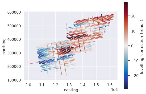
[27]:
# plot the levelling correction
blocked_survey["levelling_correction_trend_1"] = (
    blocked_survey.upward_continued_10km - blocked_survey.levelled_trend_1
)
max_abs = vd.maxabs(blocked_survey.levelling_correction_trend_1, percentile=95)
ax = blocked_survey.plot.scatter(
    "easting",
    "northing",
    c="levelling_correction_trend_1",
    s=0.1,
    cmap=cmocean.cm.balance,
    vmin=-max_abs,
    vmax=max_abs,
)
ax.set_aspect("equal")
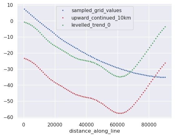
[ ]:
# look at just 1 of the leveled lines
line_df = blocked_survey[blocked_survey.line == 2]
ax = line_df.plot.line(
    "distance_along_line",
    "sampled_grid_values",
    style="bp",
    ms=2,
)
ax = line_df.plot.line(
    "distance_along_line",
    "upward_continued_10km",
    style="rp",
    ms=2,
    ax=ax,
)
ax = line_df.plot.line(
    "distance_along_line",
    "levelled_trend_0",
    style="gp",
    ms=2,
    ax=ax,
)
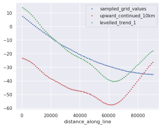
[31]:
# look at just 1 of the leveled lines
line_df = blocked_survey[blocked_survey.line == 2]
ax = line_df.plot.line(
    "distance_along_line",
    "sampled_grid_values",
    style="bp",
    ms=2,
)
ax = line_df.plot.line(
    "distance_along_line",
    "upward_continued_10km",
    style="rp",
    ms=2,
    ax=ax,
)
ax = line_df.plot.line(
    "distance_along_line",
    "levelled_trend_1",
    style="gp",
    ms=2,
    ax=ax,
)
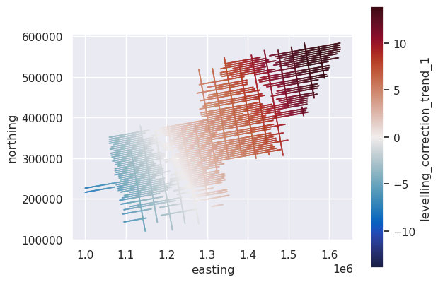
1.5. Level the entire survey to the grid#
By not supplying the groupby_column argument, instead of levelling each line in 1D, we can level the entire survey in 2D.
[32]:
blocked_survey["levelled_trend_1"] = airbornegeo.level_to_grid(
    blocked_survey,
    degree=1,
    data_column="upward_continued_10km",
    grid_column="sampled_grid_values",
)
blocked_survey["levelled_trend_2"] = airbornegeo.level_to_grid(
    blocked_survey,
    degree=2,
    data_column="upward_continued_10km",
    grid_column="sampled_grid_values",
)
blocked_survey.head()
[32]:
| distance_along_line | easting | northing | height | unixtime | grav_disturbance_filt | line | upward_continued_10km | sampled_grid_values | data_to_grid_diff | levelled_trend_0 | levelled_trend_1 | levelling_correction_trend_0 | levelling_correction_trend_1 | levelled_trend_2 | |
|---|---|---|---|---|---|---|---|---|---|---|---|---|---|---|---|
| 0 | 477.521406 | 1.000496e+06 | 226310.158049 | 4159.1 | 1.229507e+09 | 49.89 | 1 | 40.232278 | 48.675663 | -8.443385 | 42.596650 | 48.042236 | -2.364372 | 0.746947 | 67.534014 |
| 1 | 1477.462561 | 1.001484e+06 | 226460.426302 | 4160.3 | 1.229507e+09 | 50.73 | 1 | 40.972657 | 48.836891 | -7.864234 | 43.337029 | 48.749985 | -2.364372 | 0.719706 | 68.053783 |
| 2 | 2504.019094 | 1.002497e+06 | 226630.494762 | 4156.0 | 1.229507e+09 | 51.09 | 1 | 41.713109 | 49.005095 | -7.291987 | 44.077481 | 49.456755 | -2.364372 | 0.691741 | 68.570103 |
| 3 | 3518.522095 | 1.003499e+06 | 226786.791629 | 4159.6 | 1.229507e+09 | 51.07 | 1 | 42.431563 | 49.172386 | -6.740823 | 44.795935 | 50.142059 | -2.364372 | 0.664103 | 69.066650 |
| 4 | 4528.427996 | 1.004498e+06 | 226936.380167 | 4165.7 | 1.229507e+09 | 51.43 | 1 | 43.141623 | 49.342525 | -6.200902 | 45.505995 | 50.819190 | -2.364372 | 0.636591 | 69.555997 |
[33]:
# plot the levelling correction
blocked_survey["levelling_correction_trend_1"] = (
    blocked_survey.upward_continued_10km - blocked_survey.levelled_trend_1
)
max_abs = vd.maxabs(blocked_survey.levelling_correction_trend_1, percentile=95)
ax = blocked_survey.plot.scatter(
    "easting",
    "northing",
    c="levelling_correction_trend_1",
    s=0.1,
    cmap=cmocean.cm.balance,
    vmin=-max_abs,
    vmax=max_abs,
)
ax.set_aspect("equal")
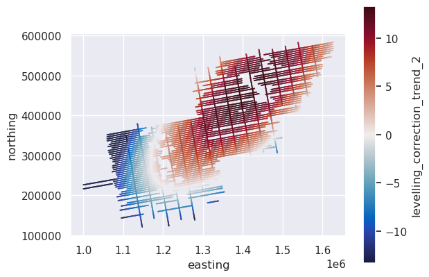
[34]:
# plot the levelling correction
blocked_survey["levelling_correction_trend_2"] = (
    blocked_survey.upward_continued_10km - blocked_survey.levelled_trend_2
)
max_abs = vd.maxabs(blocked_survey.levelling_correction_trend_2, percentile=95)
ax = blocked_survey.plot.scatter(
    "easting",
    "northing",
    c="levelling_correction_trend_2",
    s=0.1,
    cmap=cmocean.cm.balance,
    vmin=-max_abs,
    vmax=max_abs,
)
ax.set_aspect("equal")