Alternating cross-over levelling

In the Simple cross-over levelling notebook we levelling flight lines to tie lines, and tie lines to flight lines. Sometimes it can be useful to go back and forth, levelling lines to ties, then ties to lines, and repeating this process. This alternating levelling scheme is shown here.

%load_ext autoreload
%autoreload 2


import logging

import cmocean
import matplotlib.pyplot as plt
import pandas as pd
import plotly.io as pio
import verde as vd

import airbornegeo

# setup logging to get some additional info from the airbornegeo functions
logging.getLogger("airbornegeo").setLevel("INFO")
logging.basicConfig()
pio.renderers.default = "notebook"

Load data

This notebook uses the data and intersections dataframes from the notebook Cross-over-errors.

data_df = pd.read_csv("data/AGAP_magnetic_survey_with_intersections.csv")
data_df.head()

	easting	northing	height	line	unixtime	distance_along_line	mag	line_type	geometry	is_intersection	intersecting_line	mag_interpolation_type
0	621152.853769	159064.167598	4112.55	1	1.229500e+09	81.451091	-34.245	0.0	POINT (621152.8537692684 159064.1675975167)	False	NaN	none
1	621367.339673	159092.051982	4119.45	1	1.229500e+09	297.742539	-37.740	0.0	POINT (621367.3396726283 159092.05198233973)	False	NaN	none
2	621580.287957	159122.206492	4124.15	1	1.229500e+09	512.819231	-40.975	0.0	POINT (621580.287957101 159122.2064924852)	False	NaN	none
3	621766.100699	159150.747140	4127.50	1	1.229500e+09	700.811387	-43.430	0.0	POINT (621766.1006991526 159150.74713951774)	False	NaN	none
4	621924.954435	159176.326498	4131.00	1	1.229500e+09	861.711758	-45.300	0.0	POINT (621924.9544348937 159176.3264978113)	False	NaN	none

inters = pd.read_csv("data/AGAP_magnetic_survey_intersections.csv")
inters.head()

	line1	line2	is_buffered	geometry	easting	northing	max_dist	dist_along_line1	dist_along_line2	line1_interpolation_type	line2_interpolation_type	crossover_error_0
0	1	143	False	POINT (1158153 254083)	1158153.0	254083.0	73.980331	545768.070745	138071.419338	interpolated	interpolated	100.457282
1	1	144	False	POINT (1190820 259865)	1190820.0	259865.0	91.228123	578952.394848	131585.124971	interpolated	interpolated	32.156369
2	1	145	False	POINT (1223524 265689)	1223524.0	265689.0	77.978287	612181.969027	147253.495479	interpolated	interpolated	72.941955
3	1	146	False	POINT (1256193 271497)	1256193.0	271497.0	62.334186	645372.035002	136211.666612	interpolated	interpolated	84.130051
4	1	147	False	POINT (1288902 277249)	1288902.0	277249.0	99.009111	678599.158436	155115.067538	interpolated	interpolated	-7.734209

We wrap the loaded data and intersections into a Survey, which stores the column names used throughout this notebook (line, line_type, distance_along_line) so they don’t need to be repeated on every call below.

survey = airbornegeo.Survey(
    data_df,
    line_column="line",
    line_type_column="line_type",
    distance_column="distance_along_line",
)
survey.intersections = inters
survey

fig, axs = plt.subplots(1, 2, figsize=(10, 6))

df = survey.data[::10]
ax = df[df.line_type == 0].plot.scatter(
    "easting",
    "northing",
    c="line",
    s=0.02,
    cmap="rainbow",
    ax=axs[0],
    colorbar=False,
    title="Lines",
)
ax.set_aspect("equal")
plt.colorbar(ax.collections[0], ax=ax, shrink=0.5)

ax = df[df.line_type == 1].plot.scatter(
    "easting",
    "northing",
    c="line",
    s=0.02,
    cmap="rainbow",
    ax=axs[1],
    colorbar=False,
    title="Ties",
)
ax.set_aspect("equal")
plt.colorbar(ax.collections[0], ax=ax, shrink=0.5)

plt.tight_layout()
plt.show()

survey.calculate_crossover_errors(data_col="mag")
inters = survey.intersections
inters.head()

airbornegeo.plotly_points(
    inters,
    color_col=inters.columns[-1],
    hover_cols=["line1", "line2"],
    robust=True,
    absolute=True,
    cmap="balance",
    size=5,
    edge_width=1,
)

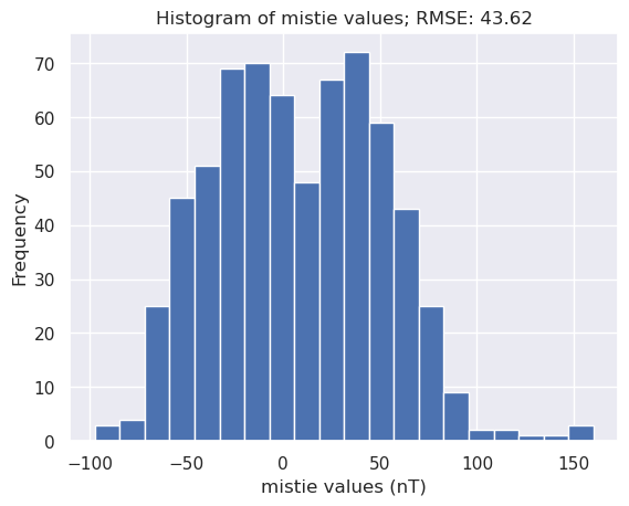
ax = inters[inters.columns[-1]].plot.hist(bins=20)
ax.set_xlabel("mistie values (nT)")
ax.set_title(
    f"Histogram of mistie values; RMSE: {round(airbornegeo.rmse(inters[inters.columns[-1]]), 2)}"
);

Alternating iterative levelling

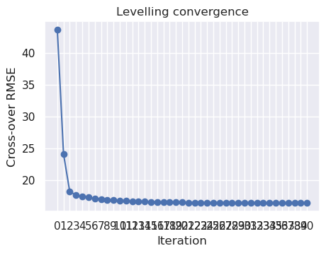
Instead of manually repeating levelling, or switching between levelling lines to ties and ties to lines, we can automate this with the function alternating_iterative_line_levelling.

This will perform up to 20 iterations where each iteration first levels the lines to the ties, then the ties to the lines. Since each iteration performs two instances of leveling, there will be up to 40 new misties columns in the intersection table. The iterations will end based on one of the following criteria:

1. the max_iterations is reached

2. the cross-over errors begin increasing instead of decreasing

3. the root mean square (RMS) of the levelling correction values for the iteration is below thhe set rms_tolerance

4. the RMS of the levelling correction values has increased more than the set rms_percent_increase_tolerance relative to the minimum RMS value for past iterations; this helps to stop run-away iterations

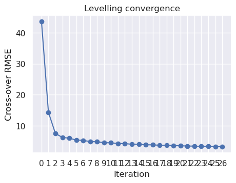
5. the RMS of the levelling correction values has not changed by more than the set rms_percent_change_tolerance between 2 subsequent iterations; this help save time by ending iterations when they aren’t offering much improvement.

survey.alternating_iterative_line_levelling(
    data_col="mag",
    levelled_col="mag_levelled_trend",
    degree=0,
    max_iterations=20,
    # rms_percent_change_tolerance=25,
    plot_dynamic_convergence=True,
)
inters_trend = survey.intersections

airbornegeo.plot_levelling_convergence(inters_trend)

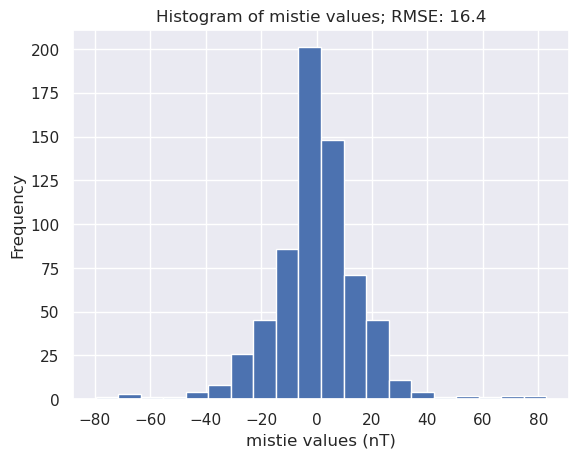
ax = inters_trend[inters_trend.columns[-1]].plot.hist(bins=20)
ax.set_xlabel("mistie values (nT)")
ax.set_title(
    f"Histogram of mistie values; RMSE: {round(airbornegeo.rmse(inters_trend[inters_trend.columns[-1]]), 2)}"
);

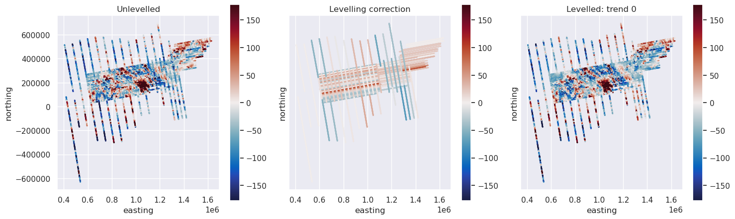
fig, axs = plt.subplots(1, 3, figsize=(15, 40))

data_df["levelling_correction"] = data_df.mag - data_df.mag_levelled_trend

max_abs = vd.maxabs(data_df.mag, percentile=95)

df = data_df[::10]

ax = df.plot.scatter(
    "easting",
    "northing",
    c="mag",
    s=1,
    ax=axs[0],
    cmap=cmocean.cm.balance,
    vmin=-max_abs,
    vmax=max_abs,
    colorbar=False,
    title="Unlevelled",
)
ax.set_aspect("equal")
plt.colorbar(ax.collections[0], ax=ax, shrink=0.1)

ax = df.plot.scatter(
    "easting",
    "northing",
    c="levelling_correction",
    s=1,
    ax=axs[1],
    cmap=cmocean.cm.balance,
    vmin=-max_abs,
    vmax=max_abs,
    colorbar=False,
    title="Levelling correction",
)
ax.set_yticks([])
ax.set_aspect("equal")
plt.colorbar(ax.collections[0], ax=ax, shrink=0.1)

ax = df.plot.scatter(
    "easting",
    "northing",
    c="mag_levelled_trend",
    s=1,
    ax=axs[2],
    cmap=cmocean.cm.balance,
    vmin=-max_abs,
    vmax=max_abs,
    colorbar=False,
    title="Levelled: trend 0",
)
ax.set_yticks([])
ax.set_aspect("equal")
plt.colorbar(ax.collections[0], ax=ax, shrink=0.1)

plt.tight_layout()
plt.show()

Repeat with wavelength-based levelling instead of trend-based

survey.intersections = inters
survey.alternating_iterative_line_levelling(
    data_col="mag",
    levelled_col="mag_levelled_filter",
    filter_type="g200000",
    max_iterations=20,
    # rms_percent_change_tolerance=25,
    plot_dynamic_convergence=True,
)
inters_filter = survey.intersections

airbornegeo.plot_levelling_convergence(inters_filter)

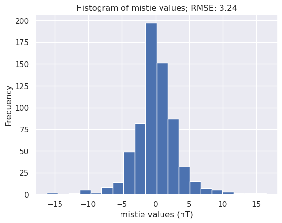
ax = inters_filter[inters_filter.columns[-1]].plot.hist(bins=20)
ax.set_xlabel("mistie values (nT)")
ax.set_title(
    f"Histogram of mistie values; RMSE: {round(airbornegeo.rmse(inters_filter[inters_filter.columns[-1]]), 2)}"
);

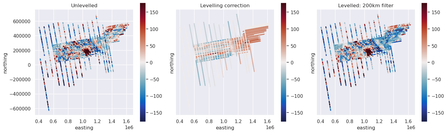
fig, axs = plt.subplots(1, 3, figsize=(15, 40))

data_df["levelling_correction"] = data_df.mag - data_df.mag_levelled_filter

max_abs = vd.maxabs(data_df.mag, percentile=95)

df = data_df[::10]

ax = df.plot.scatter(
    "easting",
    "northing",
    c="mag",
    s=1,
    ax=axs[0],
    cmap=cmocean.cm.balance,
    vmin=-max_abs,
    vmax=max_abs,
    colorbar=False,
    title="Unlevelled",
)
ax.set_aspect("equal")
plt.colorbar(ax.collections[0], ax=ax, shrink=0.1)

ax = df.plot.scatter(
    "easting",
    "northing",
    c="levelling_correction",
    s=1,
    ax=axs[1],
    cmap=cmocean.cm.balance,
    vmin=-max_abs,
    vmax=max_abs,
    colorbar=False,
    title="Levelling correction",
)
ax.set_yticks([])
ax.set_aspect("equal")
plt.colorbar(ax.collections[0], ax=ax, shrink=0.1)

ax = df.plot.scatter(
    "easting",
    "northing",
    c="mag_levelled_filter",
    s=1,
    ax=axs[2],
    cmap=cmocean.cm.balance,
    vmin=-max_abs,
    vmax=max_abs,
    colorbar=False,
    title="Levelled: 200km filter",
)
ax.set_yticks([])
ax.set_aspect("equal")
plt.colorbar(ax.collections[0], ax=ax, shrink=0.1)

plt.tight_layout()
plt.show()