Interpolating values at crossovers

This notebook shows how to interpolate your data values at crossover points.

%load_ext autoreload
%autoreload 2


import logging

import matplotlib.pyplot as plt
import numpy as np
import pandas as pd
import plotly.io as pio

import airbornegeo

# setup logging to get some additional info from the airbornegeo functions
logging.getLogger("airbornegeo").setLevel("INFO")
logging.basicConfig()
pio.renderers.default = "notebook"

Load data

This is a subset of the BAS AGAP survey over Antarctica’s Gamburtsev Subglacial Mountains. The file is downloaded and subset in the notebook AGAP_magnetic_survey.

data_df = pd.read_csv("data/AGAP_magnetic_survey_processed.csv")
data_df = data_df[
    [
        "easting",
        "northing",
        "height",
        "line",
        "unixtime",
        "distance_along_line",
        "mag",
    ]
]

# for testing limit number of lines
data_df = data_df[data_df.line.isin([149, 162, 47, 64, 80])]
data_df = data_df[
    ~(data_df.line == 47) | ~(data_df.distance_along_line.between(125e3, 134e3))
]
data_df = data_df[~(data_df.line == 64) | ~(data_df.distance_along_line > 497e3)]

# define line types: 0 for survey lines, 1 for tie lines
data_df["line_type"] = np.where(data_df.line >= 142, 1, 0)

data_df.head()

	easting	northing	height	line	unixtime	distance_along_line	mag	line_type
243447	1.078385e+06	324738.995745	4188.1	47	1.230251e+09	0.000000	-60.95	0
243448	1.078375e+06	324738.036077	4188.1	47	1.230251e+09	10.049631	-62.39	0
243449	1.078331e+06	324733.833216	4188.3	47	1.230251e+09	53.589032	-63.66	0
243450	1.078265e+06	324727.295388	4188.6	47	1.230251e+09	120.672054	-64.86	0
243451	1.078198e+06	324720.699627	4188.8	47	1.230251e+09	187.743476	-66.00	0

fig, ax = plt.subplots(figsize=(10, 10))
for _line_num, line_data in data_df.groupby("line"):
    # plot points
    ax.scatter(
        line_data.easting,
        line_data.northing,
        s=0.1,
    )
ax.set_aspect("equal")
airbornegeo.add_scalebar(ax, 100e3)

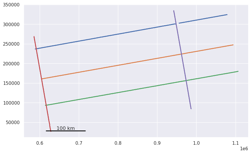
Find intersections

survey = airbornegeo.Survey(
    data_df,
    line_column="line",
    line_type_column="line_type",
    distance_column="distance_along_line",
)
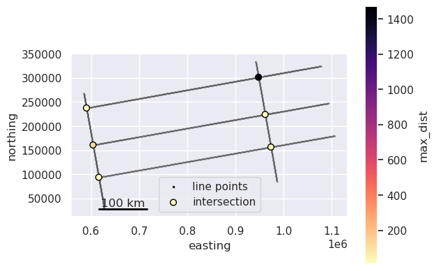
survey.create_intersection_table(method="groups", buffer_dist=200)
inters = survey.intersections
inters

ax = data_df.plot.scatter(
    "easting",
    "northing",
    color="k",
    s=0.001,
    marker=".",
    label="line points",
)
ax.legend(markerscale=100)
inters.plot.scatter(
    "easting",
    "northing",
    c="max_dist",
    s=40,
    cmap="magma_r",
    marker="o",
    edgecolor="black",
    ax=ax,
    label="intersection",
)
ax.set_aspect("equal")

airbornegeo.add_scalebar(ax, 100e3)
ax.set_aspect("equal")

Add intersections as rows to the dataframe

We can now add a row to each line of the main dataframe (not the intersections dataframe) which represents the intersection point. We don’t know the data values for the intersection point, so we will need to interpolate the data from the line data on either side of the intersection.

We need to specify the interpolation type (‘linear’, ‘nearest’, ‘quadratic’, ‘cubic’ etc.), which column we want to be interpolated (the magnetic data), and the columns containing the line identifies and the distance along the lines (used for the interpolation).

survey.interpolate_intersections(to_interp="mag", method="cubic")
inters_1 = survey.intersections
inters_1

Inspecting the intersection table below shows that we’ve added a few columns: dist_along_line1 and dist_along_line2, which show where the intersection point is located in units of distance along each line, and line1_interpolation_type and line2_interpolation_type, which inform if the data at the intersection for each line was ‘interpolate’, ‘extrapolated’, or ‘none’ (didn’t work). More on this later.

inters_1.head()

	line1	line2	is_buffered	geometry	easting	northing	max_dist	dist_along_line1	dist_along_line2	line1_interpolation_type	line2_interpolation_type
0	47	149	False	POINT (590788 237703)	590788.0	237703.0	12.785759	495443.842139	213907.289441	interpolated	interpolated
1	47	162	False	POINT (947875 301515)	947875.0	301515.0	1470.097394	135532.706601	33936.180262	interpolated	interpolated
3	64	162	False	POINT (961606 224280)	961606.0	224280.0	13.818089	134241.591186	112396.881399	interpolated	interpolated
4	80	149	False	POINT (616278 93894)	616278.0	93894.0	8.205492	497964.801259	67791.479081	interpolated	interpolated
5	80	162	False	POINT (973552 156679)	973552.0	156679.0	22.552582	135160.650024	181057.830508	interpolated	interpolated

Inspecting the data dataframe below shows that we have added 10 rows and a few columns: is_intersection contains booleans for whether the row is an intersection point, intersecting_line keep track of which line the row is intersection, and mag_interpolation_type which keeps track of the interpolationg type used for interpolating the data column we provided, in this case mag.

There are 10 new rows since we have 5 intersections, and two one is added twice (once per each intersecting line).

len(data_df[data_df.is_intersection])

10

data_df[data_df.is_intersection]

	easting	northing	height	line	unixtime	distance_along_line	mag	line_type	is_intersection	intersecting_line	mag_interpolation_type
1910	947875.0	301515.0	NaN	47	NaN	135532.706601	-163.117041	NaN	True	162.0	interpolated
7265	590788.0	237703.0	NaN	47	NaN	495443.842139	-53.886664	NaN	True	149.0	interpolated
9255	961606.0	224280.0	NaN	64	NaN	134241.591186	-32.713312	NaN	True	162.0	interpolated
16293	973552.0	156679.0	NaN	80	NaN	135160.650024	-15.720655	NaN	True	162.0	interpolated
21154	616278.0	93894.0	NaN	80	NaN	497964.801259	55.596440	NaN	True	149.0	interpolated
22324	616278.0	93894.0	NaN	149	NaN	67791.479081	83.606346	NaN	True	80.0	interpolated
24689	590788.0	237703.0	NaN	149	NaN	213907.289441	-45.204287	NaN	True	47.0	interpolated
25704	947875.0	301515.0	NaN	162	NaN	33936.180262	-139.415895	NaN	True	47.0	interpolated
26876	961606.0	224280.0	NaN	162	NaN	112396.881399	-75.259592	NaN	True	64.0	interpolated
27897	973552.0	156679.0	NaN	162	NaN	181057.830508	-0.802466	NaN	True	80.0	interpolated

We can inspect each of these interpolated intersections to make sure they worked alright. The first cell below will plot each line one at a time and wait for a keystroke to proceed to the next plot. The next cell lets you plot a single specified line.

These plots show where the intersections (diamonds) fall along the x axis of the plotted line. The y-axis shows the data value (magnetic anomaly in this case), and the vertical position of the diamond indicates the data value for the intersecting line. The vertical offset between the diamond and the line is the crossover error, which we will compute in the next notebook.

For line 162, we see the intersecting line 64 has a higher magnetic anomaly value, while the intersecting line 86 has a lower value.

# # if you want to individually inspect each line and its intersections
# airbornegeo.inspect_intersections(
#     data_df,
#     plot_variable=["mag"],
#     line_column="line",
#     x="distance_along_line",
#     # plot_all=True,
# )

# if you want to just look at 1 line
airbornegeo.plot_line_and_crosses(
    data_df,
    line=162,
    line_column="line",
    x="distance_along_line",
    y=["mag"],
    y_axes=[1],
    plot_inters=True,
)

Extrapolating values

If we look at the intersection table, we will see the intersection for lines 64 and 149 has been removed. This was because we set extrapolation to False. This intersection was beyond the end of line line 64 by ~100 m, but we allowed it as an intersection since we used a buffer_dist of 200 m. For line 64, data only exists to the east of the intersection, so interpolation doesn’t work, and it would require extrapolation. Below we show how to use extrapolation.

survey.lines_without_intersections()

inters_1

	line1	line2	is_buffered	geometry	easting	northing	max_dist	dist_along_line1	dist_along_line2	line1_interpolation_type	line2_interpolation_type
0	47	149	False	POINT (590788 237703)	590788.0	237703.0	12.785759	495443.842139	213907.289441	interpolated	interpolated
1	47	162	False	POINT (947875 301515)	947875.0	301515.0	1470.097394	135532.706601	33936.180262	interpolated	interpolated
3	64	162	False	POINT (961606 224280)	961606.0	224280.0	13.818089	134241.591186	112396.881399	interpolated	interpolated
4	80	149	False	POINT (616278 93894)	616278.0	93894.0	8.205492	497964.801259	67791.479081	interpolated	interpolated
5	80	162	False	POINT (973552 156679)	973552.0	156679.0	22.552582	135160.650024	181057.830508	interpolated	interpolated

# zoom in on buffered intersection
reg = (603e3, 607e3, 159e3, 163e3)

ax = data_df[data_df.line == 149].plot.scatter(
    "easting",
    "northing",
    color="r",
    s=5,
    label="line 149 points",
)
ax = data_df[data_df.line == 64].plot.scatter(
    "easting",
    "northing",
    color="b",
    s=5,
    ax=ax,
    label="line 64 points",
)
ax.legend()
ax.set_xlim(reg[0], reg[1])
ax.set_ylim(reg[2], reg[3])
ax.set_aspect("equal")

airbornegeo.add_scalebar(ax, 200)
ax.set_aspect("equal")

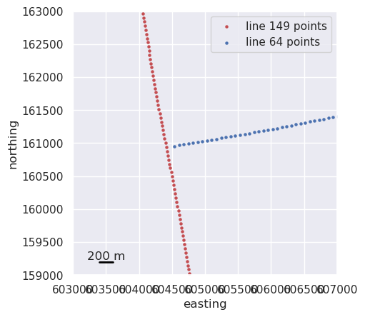
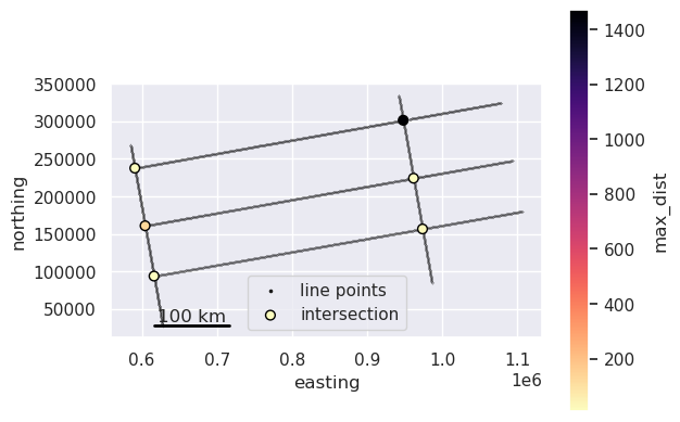
We can explicitly set extrapolate to True, which should now gives use a magnetic anomaly value for the intersection of line 64 and 149. We can view these interpolated magnetic anomaly values in profile view. We can also see in the intersection table that for line 64, the interpolation_type is now extrapolated instead of interpolated.

# Reset to baseline for second independent branch
survey.intersections = inters

survey.interpolate_intersections(to_interp="mag", method="cubic", extrapolate=True)
inters_2 = survey.intersections
inters_2

# if you want to just look at 1 line
airbornegeo.plot_line_and_crosses(
    data_df,
    line=64,
    line_column="line",
    x="distance_along_line",
    y=["mag"],
    y_axes=[1],
    plot_inters=True,
)

Windowed interpolation

When lines are really long, interpolation methods like linear or cubic may perform between using only data nearby on either side of the value to be interpolated. We can supply a window_width parameter to use this.

Different interpolation methods have a different number of minimum necessary points to perform the interpolation; for example cubic interpolation requires 4 data points and linear interpolation requires 2.

If the window width is not wide enough to capture enough data on either side, it will be doubled twice to try and capture enough data.

 - : data
 x : intersection point
[ ]: data windows for interpolation
- - - - - - -          x         - - - - - -
                    [     ] # first window
                 [           ] # doubled once
            [                     ] # doubled twice

After the second doubling, if it’s still too narrow to capture enough data, the method will fallback to one which requires fewer points. This fallback order goes from ‘user chosen method’ –> ‘linear’ –> ‘nearest’.

# Reset to baseline for third independent branch
survey.intersections = inters

survey.interpolate_intersections(
    to_interp="mag", method="cubic", extrapolate=True, window_width=500
)
inters_2 = survey.intersections
inters_2

data_df[data_df.is_intersection]

	easting	northing	height	line	unixtime	distance_along_line	mag	line_type	mag_interpolation_type	is_intersection	intersecting_line
1910	947875.0	301515.0	NaN	47	NaN	135532.706601	-163.117041	NaN	interpolated	True	162.0
7265	590788.0	237703.0	NaN	47	NaN	495443.842139	-53.886666	NaN	interpolated	True	149.0
9255	961606.0	224280.0	NaN	64	NaN	134241.591186	-32.713313	NaN	interpolated	True	162.0
14424	604414.0	160932.0	NaN	64	NaN	497099.883607	-21.091765	NaN	extrapolated	True	149.0
16294	973552.0	156679.0	NaN	80	NaN	135160.650024	-15.720641	NaN	interpolated	True	162.0
21155	616278.0	93894.0	NaN	80	NaN	497964.801259	55.596443	NaN	interpolated	True	149.0
22325	616278.0	93894.0	NaN	149	NaN	67791.479081	83.606346	NaN	interpolated	True	80.0
23421	604414.0	160932.0	NaN	149	NaN	135890.938663	-15.550791	NaN	interpolated	True	64.0
24691	590788.0	237703.0	NaN	149	NaN	213907.289441	-45.204289	NaN	interpolated	True	47.0
25706	947875.0	301515.0	NaN	162	NaN	33936.180262	-139.415895	NaN	interpolated	True	47.0
26878	961606.0	224280.0	NaN	162	NaN	112396.881399	-75.259594	NaN	interpolated	True	64.0
27899	973552.0	156679.0	NaN	162	NaN	181057.830508	-0.802471	NaN	interpolated	True	80.0

ax = data_df.plot.scatter(
    "easting",
    "northing",
    color="k",
    s=0.001,
    marker=".",
    label="line points",
)
ax.legend(markerscale=100)
inters_2.plot.scatter(
    "easting",
    "northing",
    c="max_dist",
    s=40,
    cmap="magma_r",
    marker="o",
    edgecolor="black",
    ax=ax,
    label="intersection",
)
ax.set_aspect("equal")

airbornegeo.add_scalebar(ax, 100e3)
ax.set_aspect("equal")

Interpolating other data columns at intersections

Sometimes it’s useful to interpolate multiple data columns at the intersections. Calling interpolate_intersections() again for a different column keeps any columns interpolated by earlier calls intact at the intersection rows, so you can simply call it once per column. In this case, we additionally interpolate the height variable.

# Reset to baseline for fourth independent branch (interpolating height)
survey.intersections = inters

survey.interpolate_intersections(
    to_interp="height", method="cubic", extrapolate=True, window_width=500
)

# both 'mag' (from the earlier calls above) and 'height' are now populated at
# the intersection rows
survey.data[survey.data.is_intersection].head()