Simple cross-over levelling

To start, we will perform a single iteration of cross-over levelling of the the tie lines to the flight lines, or the flight lines to the tie lines. We will use a trend order of 0, which results in a simple vertical shift of the lines to minimize the cross-over errors.

%load_ext autoreload
%autoreload 2


import logging

import cmocean
import matplotlib.pyplot as plt
import pandas as pd
import plotly.io as pio
import verde as vd

import airbornegeo

# setup logging to get some additional info from the airbornegeo functions
logging.getLogger("airbornegeo").setLevel("INFO")
logging.basicConfig()
pio.renderers.default = "notebook"

Load data

This notebook uses the data and intersections dataframes from the notebook Cross-over-errors.

data_df = pd.read_csv("data/AGAP_magnetic_survey_with_intersections.csv")
data_df.head()

	easting	northing	height	line	unixtime	distance_along_line	mag	line_type	geometry	is_intersection	intersecting_line	mag_interpolation_type
0	621152.853769	159064.167598	4112.55	1	1.229500e+09	81.451091	-34.245	0.0	POINT (621152.8537692684 159064.1675975167)	False	NaN	none
1	621367.339673	159092.051982	4119.45	1	1.229500e+09	297.742539	-37.740	0.0	POINT (621367.3396726283 159092.05198233973)	False	NaN	none
2	621580.287957	159122.206492	4124.15	1	1.229500e+09	512.819231	-40.975	0.0	POINT (621580.287957101 159122.2064924852)	False	NaN	none
3	621766.100699	159150.747140	4127.50	1	1.229500e+09	700.811387	-43.430	0.0	POINT (621766.1006991526 159150.74713951774)	False	NaN	none
4	621924.954435	159176.326498	4131.00	1	1.229500e+09	861.711758	-45.300	0.0	POINT (621924.9544348937 159176.3264978113)	False	NaN	none

inters = pd.read_csv("data/AGAP_magnetic_survey_intersections.csv")
inters.head()

	line1	line2	is_buffered	geometry	easting	northing	max_dist	dist_along_line1	dist_along_line2	line1_interpolation_type	line2_interpolation_type	crossover_error_0
0	1	143	False	POINT (1158153 254083)	1158153.0	254083.0	73.980331	545768.070745	138071.419338	interpolated	interpolated	100.457282
1	1	144	False	POINT (1190820 259865)	1190820.0	259865.0	91.228123	578952.394848	131585.124971	interpolated	interpolated	32.156369
2	1	145	False	POINT (1223524 265689)	1223524.0	265689.0	77.978287	612181.969027	147253.495479	interpolated	interpolated	72.941955
3	1	146	False	POINT (1256193 271497)	1256193.0	271497.0	62.334186	645372.035002	136211.666612	interpolated	interpolated	84.130051
4	1	147	False	POINT (1288902 277249)	1288902.0	277249.0	99.009111	678599.158436	155115.067538	interpolated	interpolated	-7.734209

We wrap the loaded data and intersections into a Survey, which stores the column names used throughout this notebook (line, line_type, distance_along_line) so they don’t need to be repeated on every call below.

survey = airbornegeo.Survey(
    data_df,
    line_column="line",
    line_type_column="line_type",
    distance_column="distance_along_line",
)
survey.intersections = inters
survey

fig, axs = plt.subplots(1, 2, figsize=(10, 6))

df = survey.data[::10]
ax = df[df.line_type == 0].plot.scatter(
    "easting",
    "northing",
    c="line",
    s=0.02,
    cmap="rainbow",
    ax=axs[0],
    colorbar=False,
    title="Lines",
)
ax.set_aspect("equal")
plt.colorbar(ax.collections[0], ax=ax, shrink=0.5)

ax = df[df.line_type == 1].plot.scatter(
    "easting",
    "northing",
    c="line",
    s=0.02,
    cmap="rainbow",
    ax=axs[1],
    colorbar=False,
    title="Ties",
)
ax.set_aspect("equal")
plt.colorbar(ax.collections[0], ax=ax, shrink=0.5)

plt.tight_layout()
plt.show()

survey.calculate_crossover_errors(data_col="mag")
inters = survey.intersections
inters.head()

airbornegeo.plotly_points(
    inters,
    color_col=inters.columns[-1],
    hover_cols=["line1", "line2"],
    robust=True,
    absolute=True,
    cmap="balance",
    size=5,
    edge_width=1,
)

ax = inters[inters.columns[-1]].plot.hist(bins=20)
ax.set_xlabel("mistie values (nT)")
ax.set_title(
    f"Histogram of mistie values; RMSE: {round(airbornegeo.rmse(inters[inters.columns[-1]]), 2)}"
);

Level lines to ties

Now we will level only the flight lines, holding the tie lines constant. We will just use a trend degree of 0, which allows only a DC shift of the lines. We will save the levelled data to a new column mag_levelled_lines_to_ties. If you don’t want to keep track on new columns, you can just use the same name as the data column.

crossover_pair_levelling updates survey.data and survey.intersections in place. Since we want to keep this branch’s intersection table around separately from the ties-to-lines branch further down, we grab a plain reference to survey.intersections right after the call, into inters_lines_to_ties – the method rebinds survey.intersections to a new object rather than mutating the old one, so this snapshot stays frozen even after later calls move survey.intersections on.

survey.crossover_pair_levelling(
    lines_to_level=survey.data[survey.data.line_type == 0].line.unique(),
    data_col="mag",
    levelled_col="mag_levelled_lines_to_ties",
    degree=0,
)
inters_lines_to_ties = survey.intersections
inters_lines_to_ties.head()

survey.plot_line_and_crosses(
    y=["mag", "mag_levelled_lines_to_ties"],
    x="distance_along_line",
    line=5,
    y_axes=[1, 1],
    plot_inters=[True, False],
    line_column="line",
)

survey.calculate_crossover_errors(data_col="mag_levelled_lines_to_ties")
inters_lines_to_ties = survey.intersections

ax = inters_lines_to_ties[inters_lines_to_ties.columns[-1]].plot.hist(bins=20)
ax.set_xlabel("mistie values (nT)")
ax.set_title(
    f"Histogram of mistie values; RMSE: {round(airbornegeo.rmse(inters_lines_to_ties[inters_lines_to_ties.columns[-1]]), 2)}"
);

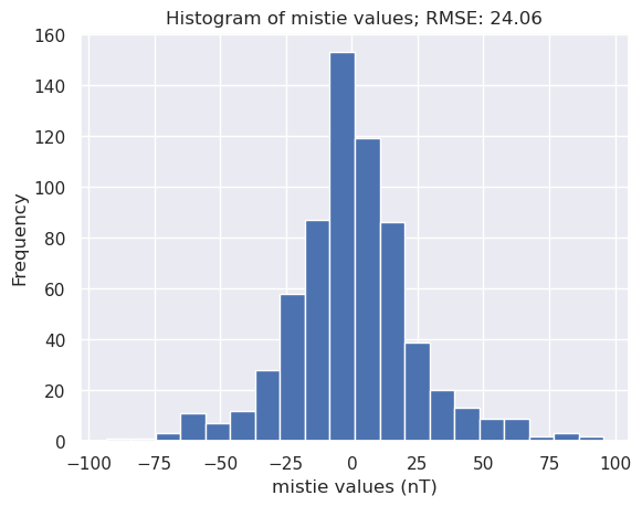
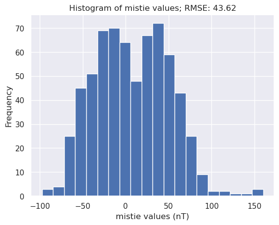
The above map, histogram and levelling convergence figures show we have reduced the cross-over errors, bringing the RMSE from ~43nT to ~24nT.

fig, axs = plt.subplots(1, 3, figsize=(15, 40))

survey.data["levelling_correction"] = (
    survey.data.mag - survey.data.mag_levelled_lines_to_ties
)

max_abs = vd.maxabs(survey.data.mag, percentile=95)

df = survey.data[::10]

ax = df.plot.scatter(
    "easting",
    "northing",
    c="mag",
    s=1,
    ax=axs[0],
    cmap=cmocean.cm.balance,
    vmin=-max_abs,
    vmax=max_abs,
    colorbar=False,
    title="Unlevelled",
)
ax.set_aspect("equal")
plt.colorbar(ax.collections[0], ax=ax, shrink=0.1)

ax = df.plot.scatter(
    "easting",
    "northing",
    c="levelling_correction",
    s=1,
    ax=axs[1],
    cmap=cmocean.cm.balance,
    vmin=-max_abs,
    vmax=max_abs,
    colorbar=False,
    title="Levelling correction",
)
ax.set_yticks([])
ax.set_aspect("equal")
plt.colorbar(ax.collections[0], ax=ax, shrink=0.1)

ax = df.plot.scatter(
    "easting",
    "northing",
    c="mag_levelled_lines_to_ties",
    s=1,
    ax=axs[2],
    cmap=cmocean.cm.balance,
    vmin=-max_abs,
    vmax=max_abs,
    colorbar=False,
    title="Lines levelled to ties",
)
ax.set_yticks([])
ax.set_aspect("equal")
plt.colorbar(ax.collections[0], ax=ax, shrink=0.1)

plt.tight_layout()
plt.show()

Level ties to lines

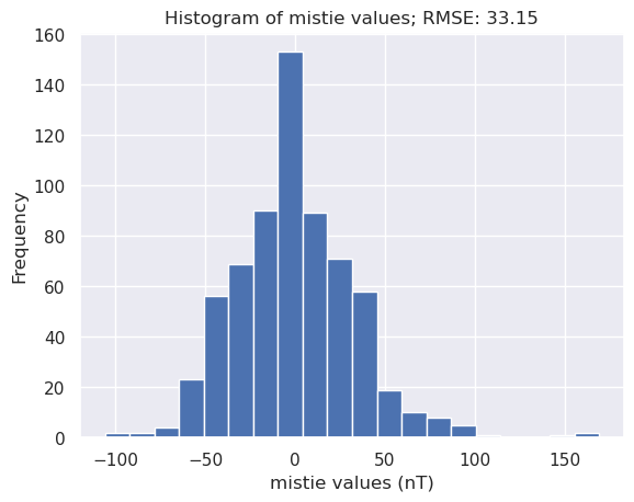
We can also level the tie lines to the flight lines. We do this be supplying the lines_to_level parameter with the names of the tie lines. We will give this levelled data a new name mag_levelled_ties_to_lines. If we want to level the ties to the already (above) levelled flight lines, we would change the data_col name from the unlevelled data (mag) to the output of the above levelling (mag_levelled_lines_to_ties).

This branch starts from the same crossover-error baseline as the flight-lines branch above (the inters table from right after calculate_crossover_errors(data_col="mag")), not wherever that branch left survey.intersections – so we reset survey.intersections to that baseline explicitly before calling the wrapper. Skipping this reset wouldn’t change the levelled values here (misties are always recomputed fresh from the current data and line geometry), but it would change which crossover_error_N columns end up in the table.

survey.intersections = inters
survey.crossover_pair_levelling(
    lines_to_level=survey.data[survey.data.line_type == 1].line.unique(),
    data_col="mag",
    levelled_col="mag_levelled_ties_to_lines",
    degree=0,
)
inters_ties_to_lines = survey.intersections
inters_ties_to_lines.head()

survey.calculate_crossover_errors(data_col="mag_levelled_ties_to_lines")
inters_ties_to_lines = survey.intersections
inters_ties_to_lines

ax = inters_ties_to_lines[inters_ties_to_lines.columns[-1]].plot.hist(bins=20)
ax.set_xlabel("mistie values (nT)")
ax.set_title(
    f"Histogram of mistie values; RMSE: {round(airbornegeo.rmse(inters_ties_to_lines[inters_ties_to_lines.columns[-1]]), 2)}"
);

fig, axs = plt.subplots(1, 3, figsize=(15, 40))

survey.data["levelling_correction"] = (
    survey.data.mag - survey.data.mag_levelled_ties_to_lines
)

max_abs = vd.maxabs(survey.data.mag, percentile=95)

df = survey.data[::10]

ax = df.plot.scatter(
    "easting",
    "northing",
    c="mag",
    s=1,
    ax=axs[0],
    cmap=cmocean.cm.balance,
    vmin=-max_abs,
    vmax=max_abs,
    colorbar=False,
    title="Unlevelled",
)
ax.set_aspect("equal")
plt.colorbar(ax.collections[0], ax=ax, shrink=0.1)

ax = df.plot.scatter(
    "easting",
    "northing",
    c="levelling_correction",
    s=1,
    ax=axs[1],
    cmap=cmocean.cm.balance,
    vmin=-max_abs,
    vmax=max_abs,
    colorbar=False,
    title="Levelling correction",
)
ax.set_yticks([])
ax.set_aspect("equal")
plt.colorbar(ax.collections[0], ax=ax, shrink=0.1)

ax = df.plot.scatter(
    "easting",
    "northing",
    c="mag_levelled_ties_to_lines",
    s=1,
    ax=axs[2],
    cmap=cmocean.cm.balance,
    vmin=-max_abs,
    vmax=max_abs,
    colorbar=False,
    title="Ties levelled to lines",
)
ax.set_yticks([])
ax.set_aspect("equal")
plt.colorbar(ax.collections[0], ax=ax, shrink=0.1)

plt.tight_layout()
plt.show()

Below we will plot the profile of a single line. The blue line shows the unlevelled data, and the orange line shows the levelled data. The blue diamonds show the magnetic anomaly values at the cross-over points. This line only had 5 cross-overs, all at the end of the line. Most of these cross-over points had high anomaly values than the corresponding point on the tie lines, causing the levelling to shift the line up vertically by ~25 nT.

survey.plot_line_and_crosses(
    y=["mag", "mag_levelled_ties_to_lines"],
    x="distance_along_line",
    line=200,
    y_axes=[1, 1],
    plot_inters=[True, False],
    line_column="line",
)